Integral and Differential Nonlinearity (INL/DNL)
Contents
- What are Integral and Differential Nonlinearity?
- How do we measure it?
- Test Methodology
- Results
- Why does the DNL Spike?
- Conclusion
- References
What are Integral and Differential Nonlinearity?
In an ideal ADC, a range of input voltages produces the same digital output value. In ideal ADCs, the size of the range of voltages that produces the same output value is precisely the same for every step. In real ADCs, this is not the case.
Differential nonlinearity is the deviation of each step from the ideal ADC step size. If the DNL for every step is less than one, then there are no missing outputs; if the width of a step is greater than one, that means that can mean that other outputs never appear.
DNL is calculated as:
\[\mathrm{DNL}(\mathrm{i})=\frac{V_{\text {out }}(i+1)-V_{\text {out }}(i)}{\text { ideal LSB step width }}-1\]
Integral nonlinearity is the deviation of a particular output code from the ideal. For example, if your 12 Bit ADC has an INL of 10 LSBs, you know that the output it reports is always within $10/2^{12} = 0.25\%$ of the “true” output code.
How do we measure it?
INL and DNL can be measured by applying a full-scale sine wave to the input and recording a lot of points. We can calculate the number of points required with the formula below, where $N$ is the number of ADC bits, $Z$ is the two sided Z-score for the confidence level we want (2.576 for 99%), and $\beta$ is the DNL resolution.
\[M=\frac{\pi 2^{N-1} Z^{2}}{\beta^{2}}\]In the testing, 10 Million points were collected, giving 0.07 LSB accuracy at a 99% confidence level (0.05LSBs at 95%)
DNL Calculation
We can calculate the DNL by comparing the number of times we saw a particular output to the number of times we expected to see it; if we saw more hits than we expected, then that output code is wider than it should be. Or more input voltages correspond to that output than we expect. Vice-versa, if it is smaller than we expect, then it has fewer voltages than we expect to map to that voltage.
The probability of a particular code being hit for a sine wave is below. Where $N$ is the number of bits in the ADC, $n$ is the code, the ADC input is $\pm V_\mathrm{FS}$, and the sine wave has an amplitude of $A$:
\[p(n)=\frac{1}{\pi}\left[\sin ^{-1}\left[\frac{V_{\mathrm{FS}}\left(n-2^{N-1}\right)}{A \times 2^{N}}\right]-\sin ^{-1}\left[\frac{V_{\mathrm{FS}}\left(n-1-2^{N-1}\right)}{A \times 2^{N}}\right]\right]\]We can calculate the DNL as, with the below equation, where we caculate the expected number of hits for that code based on the total number of samples collected times the probability of that code:
\[\mathrm{DNL}(n)=\frac{\text{# of hits}_\text{Actual}}{\text{Total # of hits} \times p(n)}-1\]INL calculation
The INL is the integral of the DNL; it can be calculated as:
\[\mathrm{INL}(n)=\sum_{i=0}^{n} \mathrm{DNL}(i)\]The problem you can run into is the INL measurement error is much higher than the DNL measurement error. The errors in DNL measurement are (approximately) normally distributed, so as you integrate the DNL, the error will grow with the root sum of squares of the accuracy above. The accuracy at the highest code is:
\[\text{INL Accuracy} = \sqrt{2^N \times M^2}\]We can calculate the INL accuracy for this test as:
\[\text{INL Accuracy} = \sqrt{2^{12} \times {0.07 \text{ LSB}}^2} = 4.48 \text{ LSB 99% confidence}\] \[\text{INL Accuracy} = 1.09 \text{ LSB 50% confidence}\]Test Methodology
I generated a 1kHz sine wave with a Rigol DG4000 function generator. I used the following code to sample the ADC at its full rate (500ksps) then dump the samples out the USB serial interface:
// Code modified from https://github.com/raspberrypi/pico-examples/blob/master/adc/adc_console/adc_console.c
#include <stdio.h>
#include <inttypes.h>
#include "pico/stdlib.h"
#include "hardware/gpio.h"
#include "hardware/adc.h"
#include "hardware/dma.h"
#define N_SAMPLES 100000
uint16_t sample_buf[N_SAMPLES];
int main() {
stdio_init_all();
// DMA setup:
uint dma_chan = dma_claim_unused_channel(true);
dma_channel_config cfg = dma_channel_get_default_config(dma_chan);
channel_config_set_transfer_data_size(&cfg, DMA_SIZE_16);
channel_config_set_read_increment(&cfg, false);
channel_config_set_write_increment(&cfg, true);
channel_config_set_dreq(&cfg, DREQ_ADC);
adc_gpio_init(26);
adc_init();
adc_select_input(0);
adc_set_temp_sensor_enabled(false);
adc_fifo_setup(true, true, 1, false, false);
// Set SMPS_MODE Pin
gpio_init(23);
gpio_set_dir(23, GPIO_OUT);
gpio_put(23, 0); // 0 for PSM; 1 for PWM
// Capture samples then ship them out over USB
while (1) {
adc_fifo_drain();
dma_channel_configure(dma_chan, &cfg, sample_buf, &adc_hw->fifo, N_SAMPLES,true);
adc_run(true);
dma_channel_wait_for_finish_blocking(dma_chan);
adc_run(false);
printf("Done\n");
for (int i = 0; i < N_SAMPLES; i = i + 1) {
printf("%03x\n", sample_buf[i]);
}
}
return 0;
}Results
Analysis code
import matplotlib.pyplot as plt
from scipy.optimize import minimize
import numpy as np
def sin_pdf(bits, amp, shift):
vfs = 1
pdf = list()
for n in range(2**bits - 1):
n += shift
res = (1/np.pi)*(np.arcsin((vfs*(n-2**(bits-1)))/(amp*2**bits))-np.arcsin((vfs*(n-1-2**(bits-1)))/(amp*2**bits)))
pdf.append(res)
return pdf
if __name__ == "__main__":
import json
dat = np.load("your-datafile.npz") # data in a 1d array called 'data_v'
hist, bin_edges = np.histogram(dat['data_v'], bins = list(range(2**12)), density=True)
bin_edges = bin_edges[:-1]
# Caculate best fit params
minf = lambda inp: np.sum(np.nan_to_num((np.asarray(hist) - sin_pdf(12, inp[0], inp[1]))**2))
res = minimize(minf, (0.5, 0))
# Plot Histogram
fig = plt.figure()
bars = plt.bar(bin_edges, hist/np.sum(hist), width=1, linewidth=1, color='blue', alpha=0.5, label="ADC Data")
plt.title("Sine Histogram Actual vs. Fitted")
plt.xlabel("ADC code")
plt.ylabel("Code probability")
# Set bar edges so you can see them at low zoom
for bar in bars:
bar.set_edgecolor("blue")
bar.set_linewidth(1)
bars = plt.bar(range(2**12-1), sin_pdf(12, res.x[0], res.x[1]), width=1, color='red', alpha=0.5, label="Fitted Data")
for bar in bars:
bar.set_edgecolor("red")
bar.set_linewidth(1)
plt.tight_layout()
plt.show()
fig = plt.figure()
plt.plot(range(2**12-1), (np.asarray(hist) / sin_pdf(12, res.x[0], res.x[1]))-1, color='red')
plt.title("ADC DNL")
plt.ylabel("DNL (LSBs)")
plt.xlabel("ADC code")
plt.show()
fig = plt.figure()
plt.plot(range(2**12-1), np.cumsum(np.nan_to_num((np.asarray(hist) / sin_pdf(12, res.x[0], res.x[1]))-1, nan=0.0, posinf=0.0, neginf=0.0)), color='red')
plt.title("ADC INL")
plt.ylabel("INL (LSBs)")
plt.xlabel("ADC code")
plt.show()Histogram
DNL
DNL is around 1 LSB except for the code transitions of the second from the second-largest bit, at 512, 1536, 2560, and 3584 counts, where it spikes to 8.9 LSBs.
INL
The peak positive INL is 6.23 LSBs, and the peak negative INL is 7.85 LSBs. A real specification would need to guardband this with the confidance level calculated above (4.48 LSB 99%, 1.09 LSB 50%).
Why does the DNL Spike?
Backround
The ADC in the RP2040 is what’s known as a Successive-approximation ADC. To tell what the input voltage is, it generates a voltage with a digital to analog converter (DAC) and checks if the input voltage is larger or smaller than the generated voltage with a comparator. By iterating through all the DAC bits, you can narrow the voltage down until you know what it is. Below is a gif (from Wikipedia) that shows how this works:
Here is the block diagram of the Pico ADC from the datasheet:
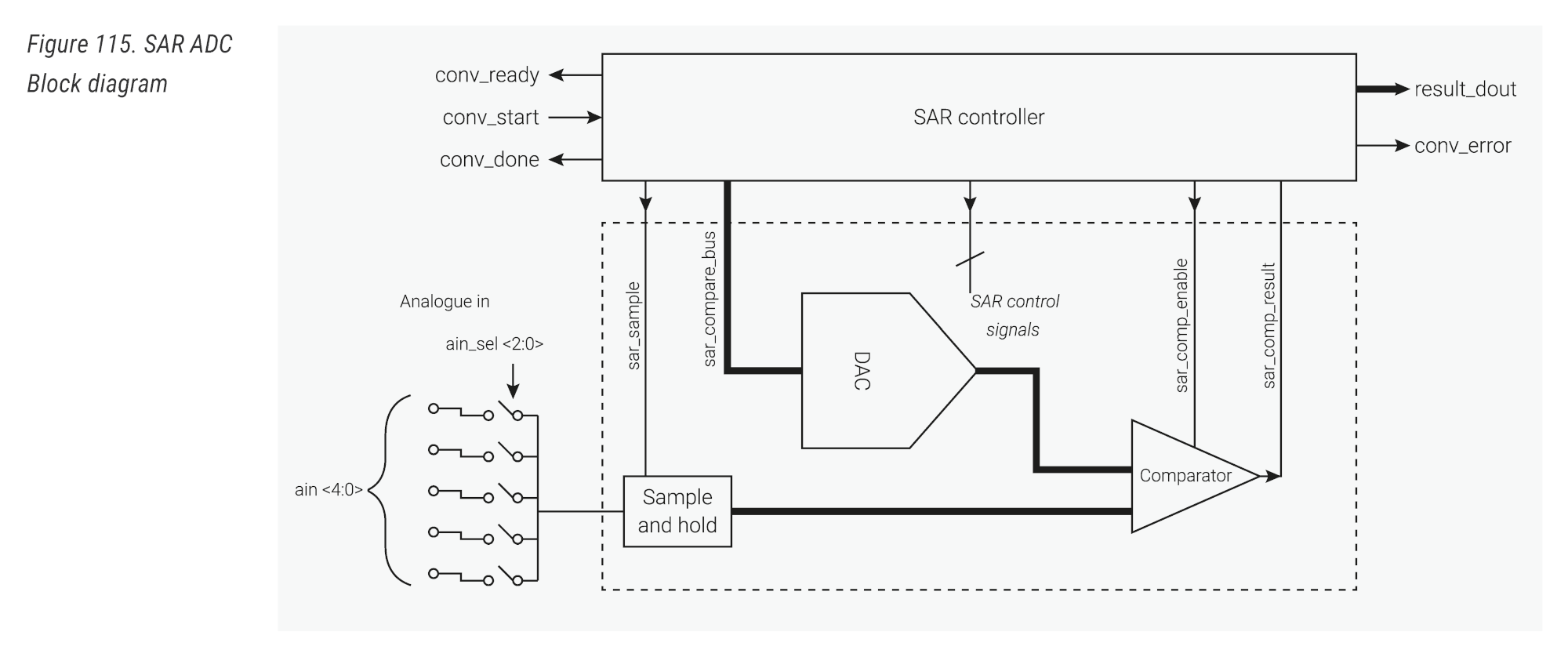
Most SAR DACs are implemented using capacitors with binary-weighted sizes, with every capacitor half the size of the last. The ratio of the capacitor sizes sets the DACs INL and DNL.
Simulating the DAC to find out what’s wrong
We can simulate a binary-weighted DAC with non-ideal size ratios between elements and try to fit the pattern of DNL we saw from the ADC using SciPy’s minimize function.
DAC DNL Fitting Code
from scipy.optimize import minimize
import matplotlib.pyplot as plt
import numpy as np
real_dnl = np.asarray(
[
float(i)
for i in """0
-2.692022315713349379e-02
1.196555299846810971e-01
7.805666751508844037e-02
1.074795231732794676e-02
3.000883091919992474e-02
3.451945303612502514e-02
-7.031634111406566134e-01
1.004782979518199504e-01
8.289202938835638079e-02
3.037437196763281833e-02
2.120296714877878408e-02
-3.771021157330967100e-03
3.889531624499675821e-02
6.206325082957087069e-02
-5.067529197916903483e-01
1.023014008916558470e-01
9.235993376192186410e-02
1.003257222772189206e-01
8.407851743317462656e-02
5.065397732913012874e-02
8.981917940776251719e-02
5.996601727014883032e-02
-7.032780934997675537e-01
6.755130840957357385e-02
1.204747606660572234e-01
8.230808270422929063e-02
7.678120717355607638e-02
-1.168739811543673124e-02
4.451820076477375210e-02
4.726631013894744271e-02
-6.011820318842755473e-01
8.569083381262809773e-02
8.496833377670642840e-02
8.429002076811187294e-02
1.071828698879331299e-01
5.324796873670956110e-02
1.101364414876977449e-01
7.796111321185983378e-02
-7.080200285040343378e-01
5.398086817137426330e-02
9.716914965219847211e-02
1.231504316146265765e-01
1.021618826053658502e-01
3.192636341732568717e-02
9.443739239898496507e-02
8.426173817040605307e-02
-4.976071284440366504e-01
8.870777481740654835e-02
1.008174643348300759e-01
1.061855869121470786e-01
9.676831934913909805e-02
4.981101640642315864e-02
4.676451190835462235e-02
1.827371006082567639e-02
-7.067828079084058635e-01
1.560100139355169446e-02
8.963333236384896097e-02
4.972496607863496898e-02
8.942193584900559600e-02
4.697049526467433900e-02
9.324866114845176135e-02
1.061125915079208504e-01
-6.841420076090778402e-01
5.886049790492675626e-02
1.111947787501001983e-01
1.218305607432792481e-01
1.489239101840313939e-01
6.061031606167022190e-02
5.217221708552721715e-02
7.797981595122083220e-02
-6.941019481653674106e-01
7.556254723038402510e-02
1.070449845594592109e-01
1.029700722488238185e-01
9.592985410823762216e-02
4.835724352146009153e-02
1.073593334674074473e-01
9.080969762980450888e-02
-5.093292733000184258e-01
8.838894644960104685e-02
8.821861317886003917e-02
9.783768917368296236e-02
9.511970383018275577e-02
8.075973142012160544e-02
9.602261646308773990e-02
4.510763178063470491e-02
-7.138614991593674741e-01
6.347183038586168280e-03
6.651990253235329220e-02
6.858293380809588058e-02
1.098349569789538460e-01
2.194888590714372256e-02
7.643215562627392323e-02
5.836100917693576307e-02
-5.645468286834049998e-01
9.926862492093713186e-02
1.287102689337791261e-01
1.072274018545831265e-01
9.137360545000650092e-02
1.510133706096317141e-02
8.868703231907537621e-02
9.432356974036082420e-02
-6.941375110600509490e-01
8.143525345585733710e-02
1.143460257209907294e-01
8.292176548629526245e-02
1.008094273412052377e-01
4.497313118733892168e-02
1.219484957812702053e-01
9.552486648527791502e-02
-4.884805393660494044e-01
9.046476291513871892e-02
8.506430144834209450e-02
7.637930407445736591e-02
1.328198329009788736e-01
5.732324478128325573e-02
9.281709371642943296e-02
8.399107945155637189e-02
-7.019555763635478840e-01
1.668811616225562844e-02
1.035803096855358874e-01
1.149891470161779061e-01
9.612605965034282107e-02
6.427241977133779649e-02
1.022835010703331271e-01
-3.699746436742257227e-02
-9.045352200915397489e-01
3.798303311618300704e-02
6.167327158495594652e-02
4.782277060851902739e-02
1.194091320187091743e-01
4.308256126368603667e-02
7.699858920286328789e-02
6.785349971728726892e-02
-7.252422268585183573e-01
2.917649430471414007e-02
8.233328029988173924e-02
7.661751744155442800e-02
1.206798629786136612e-01
9.065914321317269930e-02
1.307699462731133355e-01
6.283016208995473306e-02
-5.103637727897516463e-01
5.579463627393632663e-02
5.408710528485149993e-02
9.431966534633762222e-02
1.374135523313306795e-01
7.365088430793020891e-02
1.180893638785689426e-01
1.021140428162130576e-01
-7.068599996901079319e-01
3.958705231340964303e-02
9.215575556219435249e-02
8.725629370052612188e-02
1.365545113797381749e-01
6.519684208161113936e-02
1.331939278838156770e-01
8.956937695052480386e-02
-5.695125149680884125e-01
8.968023345413245195e-02
1.011911480999105883e-01
9.092126944315936932e-02
1.114978412861928891e-01
4.109744500485490448e-02
1.220565492087799520e-01
6.441089607960570618e-02
-6.920990315915929170e-01
4.756116591331971399e-02
9.762785072011892495e-02
9.662261268173755191e-02
9.095146859430869313e-02
6.121992891581506946e-02
1.231685880079096407e-01
1.202963800650937998e-01
-5.165126922823652933e-01
5.832413273583769708e-02
7.348662136644690257e-02
3.545128676757269837e-02
1.221320352006933785e-01
4.573123376714405275e-02
7.546957199771342495e-02
4.542086090945485211e-02
-7.054642536994786273e-01
4.981216891088990906e-02
1.193268735883041831e-01
4.585378834004827375e-02
7.242957788473547431e-02
4.634368750776651780e-02
7.895081206820364628e-02
1.024994197409128116e-01
-6.432475866467189940e-01
1.012015231241663038e-01
9.901541540341729508e-02
9.707034006029080508e-02
6.742260032091351718e-02
2.909568640505511006e-02
9.848445827905849548e-02
8.953582753248734427e-02
-7.098131945420114164e-01
7.893606898375571390e-02
1.006684947092468807e-01
1.266628637582836170e-01
1.164564147044404585e-01
5.635951886571999303e-02
9.079151902653004313e-02
7.052998794972897834e-02
-4.890138830172962026e-01
7.769556774710073555e-02
1.325223287307584208e-01
8.911063188409840130e-02
1.177248018029026788e-01
7.404790727198529154e-02
1.078632158681533948e-01
5.792178976719131178e-02
-7.104748372987593763e-01
3.813460886063313460e-02
1.124498103721809361e-01
9.291473299133379271e-02
1.166956553443485589e-01
5.615143476327544292e-02
1.278871614483421126e-01
8.193154293487681095e-02
-5.702803325924634681e-01
7.334735928724489540e-02
1.225062472681734960e-01
9.312440203693217455e-02
1.033460815552893486e-01
4.368161427447514455e-02
1.191406079888224223e-01
7.078439659853730248e-02
-6.925042917914834284e-01
3.351218535853095482e-02
8.119869717538619192e-02
7.352104064959541496e-02
9.901102061552014000e-02
4.753737825839232656e-02
1.060939314111686294e-01
6.523764897338302227e-02
-4.869920068230838561e-01
4.222880572246934250e-02
8.180546590311221777e-02
6.297433516053430047e-02
9.086484369158176477e-02
3.632160487904667612e-02
1.090943028947026772e-01
2.867208295641998639e-02
-6.970908433806405347e-01
6.878472382091671555e-02
1.064600041147094611e-01
1.131549355803982415e-01
1.294282884517929944e-01
6.505846952110694303e-02
7.508314669449167589e-02
7.892670238080601308e-02
-1.730765275057489783e-01
1.211901241104957894e-01
1.038863038547919171e-01
8.525722511963240713e-02
1.150853773337598973e-01
1.083060708565510843e-01
1.118612780547931784e-01
6.063826125949445256e-02
-7.107949051025634901e-01
4.733908116099572183e-02
1.074184713581480821e-01
8.146004452610222657e-02
1.163797369266048598e-01
5.564475625001863435e-02
1.212152830652093449e-01
9.473601397768982579e-02
-5.276453769360938129e-01
1.052220849436691363e-01
1.193006910240117513e-01
8.969987983764160511e-02
8.639131861865378958e-02
3.726175907654227792e-02
1.242938252487313378e-01
7.148272472720318405e-02
-7.017802458036934699e-01
5.848806483756141539e-02
8.072626963791629251e-02
1.128008964133337955e-01
1.156043509454700580e-01
3.245110482128321649e-02
9.960304614069714901e-02
8.105615432045110147e-02
-5.566325741341613398e-01
8.651729864143642423e-02
1.169229008678216442e-01
7.580587025926366351e-02
1.115612372153380605e-01
6.300295105427156095e-02
1.014857186039561654e-01
7.200127841129955186e-02
-7.332427975922419794e-01
4.437587379027418955e-02
6.335029577512840682e-02
9.440515172992225423e-02
1.041274636963673839e-01
5.387005386856791311e-02
9.006405337114498089e-02
7.491756157860685050e-02
-5.214944301517985270e-01
8.661694625298577144e-02
9.501382593925744580e-02
6.554170421009741787e-02
6.747883924317976678e-02
5.075322578428931308e-02
8.833555437263074239e-02
3.278194613388052403e-02
-7.157779401624788651e-01
5.972423662502235331e-02
1.231457223406100532e-01
8.679425242858984646e-02
1.524819994639254883e-01
5.837750902797211872e-02
1.114789169034748895e-01
6.935830779037255311e-02
-6.886609062520286928e-01
7.243090296663323713e-02
6.670139774827266166e-02
9.765197576225803644e-02
7.736348336576104323e-02
8.201167807391773756e-02
1.203957515513096599e-01
7.008388903841056283e-02
-6.854649172238251875e-01
8.355154622345706272e-02
8.680598911794024097e-02
7.430490813991430521e-02
1.073464392800544953e-01
4.110197965419648547e-02
1.008973958641581348e-01
1.055710408226047115e-01
-5.039306757956695249e-01
1.029316989055730769e-01
9.947501207824305247e-02
1.002501564026332392e-01
1.027929446650734935e-01
5.848142676735035295e-02
1.419999110320910862e-01
6.059473859493369474e-02
-7.102658157469308176e-01
4.270998550789317783e-02
8.624848331710910365e-02
8.445609812912269199e-02
1.181200064900460589e-01
4.532416410802508899e-02
1.185233004787868971e-01
7.501748899400384474e-02
-5.512865816673921948e-01
8.356536168080053173e-02
9.795593988800388452e-02
9.538608269203652235e-02
1.159698594622398105e-01
2.714415390698676767e-02
1.035673854497252133e-01
8.425247213804976099e-02
-7.114957296845760837e-01
6.658602081911402237e-02
9.381870729537822307e-02
1.032196561781124622e-01
1.133693865362039865e-01
4.409628346848060154e-02
9.120729187876919219e-02
7.273633591445349822e-02
-4.841001530997498525e-01
4.447048413150378465e-02
8.442483319294313837e-02
5.329279013400434195e-02
1.173455159330822895e-01
2.516672674328113146e-02
1.104279093455680094e-01
2.578916028343858358e-02
-6.972365003679816819e-01
4.162440318469617928e-02
1.291538813626917914e-01
6.347247141548240101e-02
1.027609247748098031e-01
1.859222761281076330e-02
1.020053398020170921e-01
-3.961495645684920408e-02
-8.999908190861625190e-01
3.013670663972112251e-02
1.131841323242495090e-01
1.171094883709498102e-01
1.048571744630792946e-01
6.054762648254463642e-02
1.289084519880880908e-01
5.883624026640177362e-02
-7.175973764256371457e-01
6.504539754328408918e-02
7.535260407562693885e-02
5.798635390686701641e-02
1.119730505155982492e-01
4.631355024128169795e-02
8.936114263348104991e-02
1.103994431146531063e-01
-4.968232861831826108e-01
1.224318886993103206e-01
9.424189644605429628e-02
9.660511976457164529e-02
1.100811092123035184e-01
3.765434251468358084e-02
1.029294917433478673e-01
4.070611443115801364e-02
-7.082678723099268270e-01
7.958554705993137190e-02
9.541788631742131876e-02
9.544875746731085187e-02
1.039791479335072655e-01
5.525262297948718704e-02
1.137212126511912835e-01
1.102634476483248527e-01
-5.551085282613225091e-01
1.382884450976211710e-01
9.048143305609990250e-02
1.118910848755798604e-01
7.876039574407300847e-02
5.882472791481596630e-02
8.377202960140395227e-02
6.731097831197208059e-02
-6.942311787647542642e-01
5.308475681048085981e-02
1.036151750976810337e-01
6.784493579625694437e-02
1.342130591702068720e-01
2.952097682227439179e-02
1.117365985037237497e-01
9.592208230738474839e-02
-4.753602898516237074e-01
7.919951429024796319e-02
7.594885655678651482e-02
9.050627637484098820e-02
1.054855962974521333e-01
4.510402880585329122e-02
9.342243783269932322e-02
5.237997995896437331e-02
-7.102751584974751342e-01
9.472656936290135832e-02
1.121692485630798597e-01
7.375933890395725001e-02
8.921021040886278897e-02
5.589281586929750745e-02
8.536137977715285707e-02
8.082061305043741761e-02
-6.554180261508213423e-01
2.110726523554418144e-02
1.185688733206848866e-01
9.350909731155576665e-02
8.128349581291383075e-02
6.782109194523444629e-02
1.188879064988062062e-01
3.070997633151040240e-02
-7.105411304469800848e-01
6.142446804294854346e-02
9.687053094292230604e-02
3.750892936083904949e-02
1.014003190102850116e-01
4.192263912379656787e-02
1.303283210098331590e-01
7.686267312001993091e-02
-4.899832385105693522e-01
1.176292607758329112e-01
1.150054904812962686e-01
8.173493130087750025e-02
1.101412841804036979e-01
5.346836040145030999e-02
1.056543156203300082e-01
6.075584354033103374e-02
-7.131216964539833780e-01
3.642602040038545042e-02
8.754258508863776989e-02
7.660622395210059388e-02
1.138415185517653860e-01
4.270662764923760513e-02
1.245413422142229720e-01
5.162757019830244154e-02
-5.249741208946563376e-01
3.160214158044150068e-02
1.195094355840815581e-01
1.043499967643461979e-01
1.049268579060442796e-01
7.560058765169541672e-02
1.297664632393318307e-01
5.006358251964115880e-02
-6.964432748668634154e-01
4.526164581895719685e-02
1.083406481642352759e-01
1.068142295737688485e-01
8.146297815052716551e-02
7.112073023218190571e-02
1.277348081888711739e-01
6.922647067361831219e-02
-4.569528585424952327e-01
6.773308333418470717e-02
1.304105963327919504e-01
6.201806064146730968e-02
1.264763267364352739e-01
6.764265131915681017e-02
5.380760468835443788e-02
4.838355304553609848e-02
-6.900715286597214337e-01
5.186751817514156926e-02
1.508919471517569111e-01
4.688534346826545018e-02
1.172574574205647036e-01
5.714042003529118396e-02
1.106584680990401193e-01
4.915418550610128889e-02
8.904343828331693800e+00
1.168638397077250701e-01
1.335533988254777871e-01
1.055186465352129233e-01
3.136817525100132897e-02
6.381463771197370960e-02
6.213252890848042220e-02
8.396280882790541078e-02
-7.316744888747718223e-01
2.707175676759376870e-02
8.921255038702002871e-02
7.208637058002076436e-02
9.271282073249009770e-02
5.235182769709023631e-02
7.471063257586485484e-02
3.469431516875975952e-02
-5.037716328899266571e-01
8.982530476825978383e-02
8.164330377780726344e-02
8.683112851703711499e-02
6.393533586879995845e-02
3.451288458752910238e-02
1.136821914403747247e-01
3.962977535381551064e-02
-7.212443742440453054e-01
2.219176744016038150e-02
1.172247059480262532e-01
7.117530142650818625e-02
9.637364498975853344e-02
8.504904858480255569e-02
8.241567724668064088e-02
1.168288802149752836e-01
-5.790079473772453689e-01
7.665850744484492552e-02
7.968040341444471153e-02
8.314176254560590174e-02
6.866363168898925728e-02
4.978107017901978182e-02
6.330068205192151964e-02
5.227535503835500919e-02
-7.164270577411018248e-01
6.575028075392785887e-02
6.832303061191113969e-02
8.013675525396490862e-02
9.769006353860776315e-02
1.068953769845790713e-01
9.715018090471283507e-02
6.267443562773733490e-02
-4.647290143413590480e-01
6.515974877319896663e-02
1.066516105729284902e-01
5.038027395173916290e-02
7.862947454152924287e-02
4.707311381096745961e-02
8.467361325154754148e-02
7.704390584355569338e-02
-7.054372376412371137e-01
9.464519662564963021e-02
9.278320266554040963e-02
6.241873571265599274e-02
1.090959659758590217e-01
7.557276495173370634e-02
1.227697758027914698e-01
8.027132755955435073e-02
-6.800174970345269632e-01
1.015219978604349205e-01
1.161950543541665493e-01
6.908017515103925810e-02
5.237250934470072394e-02
5.985878403375854973e-02
7.857480122471205419e-02
3.622877858823714270e-02
-6.988424500083285640e-01
6.649972539326176602e-02
7.086129840897248400e-02
1.121639310781081811e-01
6.427041271053024474e-02
4.156786452930227860e-02
9.241083060232102575e-02
4.484678960915977619e-02
-4.738183876072981082e-01
9.155362697690017093e-02
9.231905022938824423e-02
1.080323353474512693e-01
8.750031764557086866e-02
4.470966916848784223e-02
1.380410119833661575e-01
3.798495720030281575e-02
-7.336190751563385071e-01
1.940648314207038538e-02
1.134260934932607157e-01
8.503934862657391847e-02
1.227067003424773262e-01
6.782693984223353567e-02
6.399277075257692182e-02
5.375665698110343449e-02
-5.552650082857756297e-01
7.074237768497804169e-02
7.696109993243616110e-02
5.662186325591589409e-02
1.027090236009651214e-01
4.979332249882295613e-02
9.547518090862627815e-02
4.247943275288146303e-02
-7.114027404215166328e-01
3.191931305206230363e-02
5.975766123257142404e-02
7.473806070003763402e-02
9.480501476995972787e-02
4.988408401563471095e-02
9.810198166637484896e-02
5.866020646855374387e-02
-4.913417533959657524e-01
4.479929153445461054e-02
8.711972649306742866e-02
6.144642538736011517e-02
8.344827842903934645e-02
4.846498283412747909e-02
1.312430630739387372e-01
5.586346343636239276e-02
-7.120615133596718271e-01
7.860957813217317458e-02
1.113927904781546463e-01
7.674536546153509775e-02
9.885675815345917883e-02
5.064136188737422550e-02
9.140936067869187553e-02
-5.111196913340798620e-02
-9.127063135466962907e-01
6.547477193632711412e-02
9.185969311044006602e-02
4.858868466300414468e-02
9.698877640921010901e-02
4.336013304462893458e-02
9.696911084119941293e-02
5.077137800473119356e-02
-7.217764255181227107e-01
5.396914137649178045e-02
1.335499301681906115e-01
1.102850051564299161e-01
1.015702247033087868e-01
6.083879943155912073e-02
7.515493336489020848e-02
7.063786023807483438e-02
-5.011286754631946172e-01
6.111000133890542863e-02
6.837339042472079242e-02
8.934350050732620119e-02
8.008581659282221210e-02
8.831514807716889237e-02
1.178497361409389654e-01
6.170560046086381867e-02
-7.081137325419039064e-01
1.274040589214919805e-02
1.148801398706607024e-01
9.229476880206988199e-02
1.366541553562863331e-01
7.983121147404403928e-02
1.351712069012154238e-01
4.972454269264492410e-02
-5.448148047005156869e-01
8.480869876850150035e-02
6.209828582539111963e-02
5.414581811567176217e-02
9.725049755151493613e-02
5.062419877826607184e-02
1.042872914009713714e-01
4.182860277528721582e-02
-7.009970381291887875e-01
6.220590766544908945e-02
7.528405212610222996e-02
1.051497368772773555e-01
5.976255960746712503e-02
4.406895511648301067e-02
1.085307238106996142e-01
7.891338800759695182e-02
-4.799361822637420172e-01
8.016773585523195855e-02
1.173654979651879149e-01
7.323351589939330886e-02
1.066130700951488652e-01
3.108804897184036520e-02
9.486487217804073779e-02
2.648209933177425590e-02
-6.827526407511799178e-01
2.669126761775264534e-02
1.239622155181274721e-01
5.978675379880504792e-02
1.344375866408935583e-01
3.242051955646640948e-02
8.921019983233402506e-02
3.358952152353578136e-02
-6.662706665626763058e-01
5.222788743409001455e-02
8.438470477220683108e-02
8.790864594679304034e-02
9.192122152380188815e-02
6.529143738942155828e-02
1.155299874827231399e-01
4.602671656280521439e-02
-7.256794713676838482e-01
3.061358525740920378e-02
6.728084775217446634e-02
8.788136974865068396e-02
7.676193024871613702e-02
3.777880064048755315e-02
9.554666301859526811e-02
9.908276154870554464e-02
-4.915119731178847484e-01
3.760859662454141272e-02
1.008867885327093816e-01
6.521153335206575363e-02
5.254812511078665871e-02
6.440638870242243463e-02
1.086822666684115202e-01
4.345202595649966248e-02
-6.854191164545879733e-01
7.556110014488415239e-02
1.155045466007538213e-01
6.096288704840246986e-02
1.024164034384575928e-01
5.322788255852284323e-02
1.109917505671311755e-01
5.632535244263392471e-02
-5.423939671290108899e-01
3.522281725844300659e-02
1.153322152585023463e-01
5.461332432389354175e-02
8.237813237054658622e-02
3.691843456023047310e-02
1.162023706562436143e-01
6.773713961906069336e-02
-7.258616223310312421e-01
5.893622681743360125e-02
8.727928106910654016e-02
8.238465317811183297e-02
1.634239801162582495e-01
2.337086022684031761e-02
1.104284883781616600e-01
1.119984077250195664e-01
-5.141515562386240745e-01
3.096827122508649666e-02
1.092352616266381027e-01
8.836706959938034345e-02
2.707167646353858537e-02
8.499139689761880945e-02
1.140079095691861610e-01
7.261113074273395362e-02
-7.040944470198260419e-01
5.970045875019636128e-02
1.097727818541793798e-01
9.031094073097500896e-02
9.036147249075643373e-02
6.385207232800538257e-02
1.350799751965972018e-01
9.752837312521966950e-02
-4.043513814761123815e-02
1.106806143793317432e-01
1.097292117891439656e-01
5.097450691114735477e-02
7.161321128185815788e-02
3.944377404270982268e-02
8.173975895081686538e-02
7.119657510162635816e-02
-7.173301597884499392e-01
7.326463447554498742e-02
8.135950937421720930e-02
8.946115720072445043e-02
6.071465287518895693e-02
5.163800085868985867e-02
1.021833967451839520e-01
8.603733029887883355e-02
-4.987019287978207149e-01
5.369430565879329542e-02
1.134489061287262679e-01
8.055456539311611763e-02
9.324224301006611704e-02
8.971446754017975422e-02
1.085043839846029368e-01
6.843320743747716151e-02
-7.186713396279089672e-01
4.354990244199008487e-02
9.894681639205793466e-02
6.133203371131856763e-02
9.898065611533257702e-02
4.503865887026492487e-02
1.244734963940015149e-01
6.743285892328865216e-02
-5.580413253113055694e-01
8.374514317288950238e-02
8.323710896008829074e-02
6.741306724337303713e-02
7.710899198625464912e-02
2.958535144059326605e-02
1.200400668404291160e-01
1.776562699718065019e-02
-7.016909527104215893e-01
6.837356422040485882e-02
6.323801186848920786e-02
9.191467958906129887e-02
8.011885881171609824e-02
2.933275729636197759e-02
9.548733106905182844e-02
7.289315926438111326e-02
-5.069604193130484715e-01
7.285507963589177294e-02
8.877011607343465727e-02
8.412701412390122258e-02
9.954513301803702419e-02
5.320473395348979118e-02
8.252560227943428472e-02
3.870911269997701076e-02
-7.139157132504759806e-01
5.151510132036030143e-02
9.429870090205039190e-02
6.692103890132972133e-02
9.890379969509655034e-02
6.581834349463000500e-02
1.489972764762823587e-01
7.401728499294546459e-02
-6.771845839868083639e-01
1.018942211206159687e-01
9.772697958049136879e-02
4.123422517671970766e-02
8.471381966722968393e-02
7.171585868391083807e-02
1.121333547577576528e-01
4.516323766000285289e-02
-7.336613040791590823e-01
5.595691393163093608e-02
6.473704667929047751e-02
7.560337789058646507e-02
8.855863765243188190e-02
2.607738936576287081e-02
8.795210010784426657e-02
8.738650820362048321e-02
-5.003548384240006364e-01
1.102275304652720056e-01
1.159253662793928719e-01
1.268439909360465911e-01
1.048905125769614699e-01
6.046498617005280352e-02
8.286275576374402263e-02
3.890988834009712072e-02
-6.972897474678230179e-01
5.654180360660565619e-02
9.937991974675419726e-02
3.075056085521388205e-02
1.018929368393897139e-01
5.887687162921961814e-02
1.431941285809301689e-01
5.663313913174761183e-02
-5.483137476262291976e-01
9.321913030805406564e-02
1.015579697779491752e-01
5.054697838351351891e-02
9.408107628840189918e-02
8.770784542523668570e-02
1.270848744300354660e-01
5.915762517895428729e-02
-7.110177083276949528e-01
1.079658604045572456e-01
7.629286288769576707e-02
8.306635448440635727e-02
6.717240360366827367e-02
1.064845799465041765e-02
1.234674791901886337e-01
6.058311493092038980e-02
-4.723938061762631424e-01
6.093170650403312294e-02
1.195118574368845277e-01
7.766962665819687750e-02
8.022847638689034611e-02
5.156439399785428535e-02
1.367052667931569765e-01
2.223479862772781424e-02
-7.080407916799223988e-01
2.995988129440019243e-02
1.597728129379025752e-01
7.907449229078267194e-02
9.224958981995201590e-02
1.197700484101689167e-01
9.525786669367919401e-02
-3.236219921840199909e-02
-8.899606307696011909e-01
2.851064539597358838e-02
1.321350289136582479e-01
4.157709715924173821e-02
9.683554932090210343e-02
2.589754771603680616e-02
1.403406456670936997e-01
2.778125807590892116e-02
-7.226874316029897605e-01
1.064893016146783999e-01
1.021240862000460936e-01
5.664211385853890057e-02
3.729610158376939211e-02
6.602535204854120821e-02
1.033293072667298418e-01
3.263841996107097465e-02
-5.190543980582126293e-01
9.124802100045070752e-02
1.221921247053454618e-01
7.014058560423475086e-02
1.155658425135250855e-01
4.738872193715160108e-02
9.766482432178213990e-02
6.483104972919262465e-02
-7.123575384271040312e-01
2.861166426033734389e-02
8.378854637266397454e-02
5.895424806875704249e-02
8.086024582208217737e-02
9.471702146637417385e-02
1.042804784223865244e-01
4.820317464084022951e-02
-5.526748256387630232e-01
5.492667901096126570e-02
1.221278973857138350e-01
4.441196596640839545e-02
8.038982981608322476e-02
5.545088283896193460e-02
9.847236495102262843e-02
2.818255447565265470e-02
-7.213952152954102859e-01
8.729149784052592231e-02
1.357899130572297608e-01
1.221617321473205120e-01
6.255935871878182120e-02
6.133362077419479697e-02
8.662234798891765841e-02
5.725295039455113866e-02
-4.811956088407621790e-01
7.104078561430493544e-02
8.932215744327609563e-02
8.376157608756318318e-02
4.728200108941127411e-02
4.983846751920339990e-02
1.120987535800650470e-01
2.074876916392387471e-02
-7.066986020206202923e-01
6.931230075400285351e-02
1.387341100075023537e-01
6.302538874218055476e-02
7.973131876515338057e-02
1.372593757309088502e-01
9.412537357045325237e-02
7.709709113230100996e-02
-6.595401857559246572e-01
9.422483018615301908e-02
7.772085086761792994e-02
4.920701441890029670e-02
1.221389941846342531e-01
6.578743181325208411e-02
5.743505807758597648e-02
4.907593927617992513e-02
-7.104586106976928939e-01
7.113897971775839935e-02
1.158028636528225519e-01
6.151091269402053641e-02
6.462331193409576180e-02
4.858247673589044524e-02
9.001394555484498738e-02
8.054120095217376374e-02
-5.091198665399778722e-01
7.472657955947692443e-02
1.584374597054671874e-01
7.767572396488864328e-02
1.181032895004623384e-01
7.129606632881202444e-02
1.479829361116784536e-01
7.588856270193788944e-02
-7.060741085048964916e-01
2.003011566762413764e-02
5.556981953446404887e-02
5.813546537501013134e-02
7.060498324827757521e-02
1.105997275569812199e-01
1.241955701104588972e-01
8.658249398842343680e-02
-5.151945053977478040e-01
4.654721154032004371e-02
5.848289594495104105e-02
9.965456871180022880e-02
6.858486896765536578e-02
6.287871772285202887e-02
1.074041439258097697e-01
2.273647316171922839e-02
-7.143984168617183439e-01
6.377031401266375354e-02
1.393101068382702756e-01
8.384359569591692818e-02
7.203919584230611406e-02
9.010724587741059111e-02
9.766946947373433829e-02
4.266506736486430640e-02
-4.771081253401082689e-01
7.328405713819186040e-02
1.013563161271118229e-01
5.958390485741427156e-02
6.714684247138502649e-02
9.635265165325135328e-02
1.266871708682555386e-01
5.877029969386171615e-02
-7.050902779363614759e-01
3.280239553444430634e-02
6.815499309748207502e-02
6.517069176950207599e-02
8.109172620939397724e-02
4.695556464376893224e-02
1.196408173018495003e-01
1.591061804608218111e-02
-7.054290222133072774e-01
1.173947745984567081e-01
1.250018052803618662e-01
1.025140965104756052e-01
4.432668420801122444e-02
9.653529757349810225e-02
8.070957656020216753e-02
2.301474292669558608e-02
-7.297880138424736041e-01
5.215503944077615195e-02
1.010951040187575423e-01
1.031244107452340408e-01
5.819784778291658967e-02
6.524603718860455537e-02
9.858810530677253325e-02
6.592494483173361175e-02
-5.035296950704336583e-01
7.835989529406095500e-02
3.165534935243896619e-02
1.020129760821724130e-01
5.920804112921373985e-02
4.440565211740388207e-02
1.165142998132155938e-01
9.667069954919704777e-02
-7.177501688976790639e-01
7.939647521382253714e-02
1.111771192065296177e-01
8.568769013799149015e-02
8.377874837231180649e-02
6.613170179686522765e-02
8.389062496810906211e-02
7.354200813954148153e-02
-5.820383893031939593e-01
8.939952187565602948e-02
7.678953501449581331e-02
9.795433643992890183e-02
8.083210141985652797e-02
7.834708804037915364e-02
8.656778654078989277e-02
6.716937254271893032e-02
-7.169134846341664868e-01
4.130912234532746474e-02
1.138518235074168494e-01
5.323186906957499964e-02
9.702624719147046051e-02
6.912007185792101716e-02
1.259383329212728775e-01
9.237155786732764717e-02
-5.104608471849720885e-01
9.925031194313316263e-02
1.063684222055176765e-01
4.559442769783617067e-02
9.627894661738345405e-02
7.905677932342380920e-02
8.051178612047404926e-02
2.928487547500635557e-02
-7.223446417441978795e-01
8.487828672667263596e-02
1.265898792492725633e-01
8.552191766081751467e-02
1.136415814180997685e-01
4.190010569544022623e-02
1.194079155089635691e-01
3.967513281711365636e-02
-7.046477408788154317e-01
1.084641616735915193e-01
7.582647303955902807e-02
1.102502381784218333e-01
1.082998715222918129e-01
8.416390845501320328e-02
1.573091780117312766e-01
5.178411913164815417e-02
-7.335618047196560410e-01
9.966065538829615988e-02
7.833227688424426738e-02
4.445523032747122905e-02
8.864404257855662550e-02
7.527410329561567970e-02
7.159095573768725629e-02
9.528728506153738564e-02
-4.887195556696429799e-01
8.792315642164938438e-02
6.710849109324978912e-02
1.045350241743296937e-01
9.685140637997036173e-02
3.944762458692818718e-02
6.717925186025253126e-02
7.434255210281981441e-02
-7.317673861984493877e-01
5.149397179949533054e-02
1.158818989077607942e-01
1.047476133560658607e-01
1.016224373361265254e-01
9.391308043812185424e-02
1.251553145102455300e-01
7.676050677502010977e-02
-5.557625289999694740e-01
3.493158500331294825e-02
1.063369429517961873e-01
4.009628616217031372e-02
9.030925860949645667e-02
8.487090972536504019e-02
7.942897923182479225e-02
8.030102378467440793e-02
-7.116106079982313926e-01
7.055207044551736750e-02
1.007353154211523272e-01
7.861372516950160261e-02
3.405011463890339485e-02
6.252068137435751183e-02
9.273251042216590356e-02
2.683806194412574619e-02
-4.852899569036059901e-01
5.907002103493530498e-02
1.054409511621319240e-01
9.191095854117281583e-02
8.874760282786908760e-02
9.077063403369556305e-02
9.394753856671278491e-02
6.482325906702723906e-02
-6.993923477215743256e-01
6.366269753310871415e-02
2.930961854425140345e-02
7.808973171502442412e-02
6.220424891850950821e-02
8.848569755791824143e-02
7.606086931602251688e-02
-3.406310213596541736e-02
-9.225195633885008295e-01
6.766184734285007885e-02
1.408367814242967864e-01
6.128084127909061429e-02
5.287761554440373324e-02
4.620636714839609915e-02
8.412379259911251239e-02
8.151111455241277781e-02
-7.317244396419716468e-01
4.498272288771199001e-02
7.540084789664858178e-02
1.365679960271712901e-01
1.026410917259363842e-01
8.668169789098589817e-02
1.032121230354554609e-01
7.795581744076285347e-02
-4.838180891492334101e-01
3.553347252574079462e-02
8.866429304493350649e-02
7.732200733487792910e-02
5.667371959476952270e-02
6.043219167164171068e-02
1.048988675828628203e-01
7.144338633164792896e-02
-7.195618245700931004e-01
8.013583794761758305e-02
8.739517757318626678e-02
4.400063992472347252e-02
9.551677845968442604e-02
5.093620022941003356e-02
1.269526982067956666e-01
5.554532428426539603e-02
-5.948160092405883059e-01
9.456259290348367763e-02
1.566653326456288742e-01
9.452663498601721059e-02
1.117235250954407011e-01
7.405809937135710008e-02
9.768001366294454257e-02
1.502200207118931097e-02
-7.219389012197601208e-01
8.096698299195881354e-02
1.011052652998236656e-01
4.584022919253216699e-02
6.714824704536415112e-02
8.554183292280503892e-02
1.051139943654841868e-01
1.077253266599156323e-01
-4.761454982547431714e-01
3.332836614083012350e-02
1.161494717090547635e-01
9.123417873247974264e-02
8.681215374416129116e-02
3.609153252494556874e-02
1.143024774688918832e-01
6.180403033085424269e-02
-7.155719509633288178e-01
6.642213823199671907e-02
1.488210256650879248e-01
1.185794186940813955e-01
8.949681619464344706e-02
5.863832351656350639e-02
1.276045800359539850e-01
2.096044919451989230e-02
-6.856479488188954585e-01
7.022639864707436175e-02
9.810940019613356711e-02
6.896987736970361382e-02
1.121562217641538517e-01
8.829967985630249316e-02
1.126809067926117791e-01
5.526505913427826044e-02
-7.168423264203624967e-01
5.458275121708489053e-02
8.368870867295630234e-02
1.304807627961828143e-01
2.998508426025314755e-02
4.319118465837279430e-02
7.231975177834382151e-02
9.969243372823188842e-02
-5.039916120216396678e-01
8.958314149576396268e-02
1.393995361051663107e-01
9.480757605743672656e-02
4.842359917922411938e-02
8.704467414115746315e-02
1.162334095879020701e-01
2.019922858073974758e-02
-7.157915398252394645e-01
3.603146471473883672e-02
1.196181753291774008e-01
8.380512090011138504e-02
6.630896712168921070e-02
1.055924640584786633e-01
9.933421467828473794e-02
5.933949915303715628e-02
-5.282212345521464236e-01
9.238117036824622375e-02
5.650190782151054414e-02
6.917815393016768510e-02
6.764021873704439969e-02
4.891551299752294746e-02
1.291695545927324940e-01
2.329710115300986928e-02
-7.420432973003645571e-01
9.077639761452482858e-02
1.058499152646297237e-01
1.007540922741474443e-01
1.128679019847937948e-01
3.771849762659029714e-02
1.068267831841156479e-01
5.480497949928442303e-02
-4.926795425831839159e-01
6.544643997970833738e-03
9.056278471950629516e-02
8.247869214055625342e-02
8.509290155347026818e-02
6.213565717889002471e-02
1.105475816519838617e-01
5.129248198891089849e-02
-7.214989372098754572e-01
6.662766070414871677e-02
7.638325824082348170e-02
1.046022721852475357e-01
5.838285303718659947e-02
4.550394623178588560e-02
1.029301321495330601e-01
5.369934665347386726e-02
-1.117945673607292356e-01
1.477582870502338608e-01
1.235515115659773233e-01
7.249185867294305474e-02
1.007602912944061124e-01
8.846163445817278870e-02
1.256975708964382932e-01
2.444562883342449311e-02
-7.545828643997769536e-01
7.086474948533716400e-02
8.662113027889195571e-02
8.505623428109498896e-02
7.691638920846566307e-02
8.491188928547543924e-02
9.888900472274420039e-02
6.443377715607567779e-02
-5.203072218815703032e-01
9.538594897545271678e-02
7.466970521598970123e-02
9.583890292503238761e-02
3.500608276579697531e-02
8.730938273764099478e-02
7.735214634866260930e-02
6.379648145272542870e-02
-7.196178539874356073e-01
1.175632115908582520e-01
1.477588288491176183e-01
6.586467253372929598e-02
8.586804777756662510e-02
8.308985233672006032e-02
5.091798649694823098e-02
1.075268087842280451e-01
-5.727419858686755294e-01
7.676314274579798536e-02
9.919172815262178311e-02
3.696633013740435736e-02
1.098424736121959011e-01
6.261051765448955031e-02
1.439313726546402883e-01
8.466800344566971503e-02
-7.253230186742587460e-01
5.564250196600228904e-02
1.093660305002148725e-01
9.274645089245270313e-02
4.724689258149283866e-02
4.324204557904409718e-02
8.436702631908543637e-02
1.110627525737062360e-01
-4.834892042476069962e-01
1.127027317606812407e-01
1.249649194175845857e-01
6.133572022386180045e-02
1.037150493295673215e-01
1.051348977908566074e-01
1.131845585608144411e-01
2.840332055348238072e-02
-7.467684876373421599e-01
3.905276003999391676e-02
1.031885425010767854e-01
8.047615623207304836e-02
9.154484472218538116e-02
8.149442751576940758e-02
1.269735254729662532e-01
4.085353896648236116e-02
-6.968630369298997040e-01
9.198399201865758990e-02
9.400375989881282202e-02
9.421127213167412862e-02
4.184285284653554982e-02
7.407462335172376733e-02
7.548634469207793352e-02
8.596808247648590751e-02
-7.187805787867838081e-01
6.883431206616963394e-02
1.361894660988627326e-01
1.146178192575091348e-01
7.427569792914434643e-02
6.418505469815394271e-02
8.799551615764977797e-02
7.850843172584021090e-02
-4.888097969354688876e-01
5.285884746451285920e-02
9.486024980589413680e-02
5.324721343711535937e-02
9.223275871691805072e-02
4.029716136644179159e-02
1.556933093299808224e-01
2.915543551943744482e-02
-7.070283870201539145e-01
7.745839417604583055e-02
8.857655650027096428e-02
6.389140510171298359e-02
6.772626136337822622e-02
4.484895218136175643e-02
1.367288880789714334e-01
2.830707733165738205e-04
-5.541348768021956417e-01
9.602876834910634152e-02
1.174934437955208466e-01
9.155915704476136341e-02
1.087747454782155287e-01
4.817345227746439029e-02
1.450474233133378643e-01
1.266198655245664995e-02
-7.238258057962780878e-01
5.317645246513325041e-02
6.309888901418725382e-02
5.659128503321331216e-02
8.538808061472336064e-02
8.375213500259737209e-02
9.368539507026540925e-02
8.291360840129580190e-02
-4.426102462576608776e-01
2.480106656119240860e-02
8.774562761916526732e-02
7.086887071554848205e-02
9.421899833963731652e-02
4.197424566288976422e-02
6.410708789394781171e-02
4.538331425010611042e-02
-7.578246401733825799e-01
7.502833376169237845e-02
1.350143961955037053e-01
1.138470863264897659e-01
9.877646239377591009e-02
8.492138086045075696e-02
1.095314710764900834e-01
-4.235515795680044882e-02
-9.114272771966832609e-01
4.838962564309046144e-02
8.767396165036300815e-02
4.507629950357805448e-02
5.503216265164656562e-02
7.416141916261076439e-02
1.055259863774804518e-01
7.024000411748088091e-02
-7.461578767800618461e-01
8.527933887608862840e-02
1.197245378193874110e-01
7.829615731205019635e-02
9.132827148486977187e-02
4.314678630939883242e-02
9.964828051788399144e-02
5.573817041675210859e-02
-5.075678851120051238e-01
8.671373214753774761e-02
1.034339310167509129e-01
3.682133500041295804e-02
1.123744458307538441e-01
9.600505918477653111e-02
1.630085529841309722e-01
3.197717107492037414e-02
-7.277052901612383051e-01
7.586045801120944176e-02
1.122288278200276324e-01
2.528037176198427716e-02
8.988046541957750435e-02
4.647743470049436887e-02
9.943741443009157521e-02
5.233750685598193009e-02
-5.480491409562719962e-01
7.723889349333479259e-02
1.363786434339302467e-01
8.986752889011406786e-02
8.082296906342745224e-02
8.652438958208064079e-02
1.205009917012209719e-01
2.170335348994734126e-02
-7.288557014088381525e-01
5.584492273382402061e-02
1.156679113509893053e-01
8.262490006768175022e-02
1.504678855894605594e-01
1.057282017635512439e-01
8.866791559271258727e-02
1.011464403860267147e-01
-4.767362152284276844e-01
6.515972187622742773e-02
1.084290107415275539e-01
3.961954108263410212e-02
6.380201561398868293e-02
7.690215445929560190e-02
9.493530258472970829e-02
5.935857731466720466e-02
-7.164753066616442734e-01
4.920035224068142199e-02
1.171789572072103880e-01
6.246682910155931800e-02
9.469687025990003448e-02
5.415109913572124789e-02
1.363590655343260849e-01
4.336096005872436265e-02
-6.784906658954482639e-01
6.836016468011019143e-02
6.543272946759093323e-02
1.051030203926317519e-01
9.106505237750250892e-02
9.307910220417281444e-02
1.389465404403078530e-01
6.189668854142138521e-02
-7.250648695097845486e-01
9.001509133320140243e-02
9.759081778695244402e-02
5.262963961018574111e-02
5.896503748325176986e-02
7.457618786103181741e-02
9.823037938540135627e-02
3.221400934145557393e-02
-4.816534389635586111e-01
7.519846434606858310e-02
1.471260004312096026e-01
5.508677014189977683e-02
6.575949806197223246e-02
8.448189829128094352e-02
1.180673433921948234e-01
2.906573572368298386e-02
-7.436258745091979261e-01
6.466101232162180246e-02
1.069334724894011046e-01
7.239653081831920467e-02
5.148095424180665347e-02
6.030469565589946512e-02
1.335883103517931936e-01
5.998229963241064056e-02
-5.220113308125966523e-01
1.098820995690035218e-01
7.158843595740327359e-02
4.444771258250024282e-02
8.057016980807207851e-02
6.893225135441283236e-02
1.044469421247646856e-01
1.461770295004849451e-02
-7.151232145289555531e-01
4.034637269165086693e-02
1.249198419298989116e-01
8.409398945988133534e-02
8.486272690836726973e-02
5.333566664361044651e-02
1.162152476744278129e-01
5.486374007155103705e-02
-5.122615288718225246e-01
8.559744270334146421e-02
9.506584788518934737e-02
6.786361085771464019e-02
4.935694478886043512e-02
3.892762200812360796e-02
1.093321794034822769e-01
9.082263674309087875e-02
-7.126414034598760328e-01
8.675754185807793561e-02
1.435171393763461367e-01
7.273319643964115677e-02
7.038513105007959680e-02
7.488250520498329621e-02
1.142396233482072532e-01
3.843280312922581210e-02
8.668398322060829386e+00
7.419875735919911897e-02
9.925048279455639388e-02
3.835017178886346301e-02
5.966529686105292996e-02
1.083996506905950952e-01
1.384524305773915387e-01
1.645015566701935050e-02
-7.164046000891184374e-01
8.216389803565338212e-02
1.446465617165546558e-01
8.680444152603428165e-02
6.449273211207318113e-02
5.153029059798752698e-02
1.283860224718516019e-01
8.127071372520999759e-03
-4.964969321265912949e-01
7.327638832736727004e-02
9.587762021636936360e-02
9.539047870573069687e-02
7.243053556391876313e-02
8.505019986961048772e-02
1.669796547787800733e-01
-8.974770966212020085e-03
-7.120862628015844908e-01
1.043259472749196171e-01
1.082099946666079671e-01
3.649721984840170741e-02
8.848661190204620830e-02
7.299648413686110615e-02
1.056273585844182961e-01
8.825966368698034969e-02
-5.680191411936241774e-01
1.135326309068136474e-01
1.299250355424403924e-01
1.213058713678250022e-01
5.639335790828448047e-02
1.009326807023938066e-01
8.667550085642594659e-02
1.047232592972502374e-02
-7.290485300904254728e-01
5.639820213216539813e-02
9.470347075557250527e-02
8.293936705520699171e-02
7.555451864474549417e-02
9.571707193035305927e-02
1.133792542639306955e-01
6.403426646044940718e-02
-4.719919349362986516e-01
6.929399465686292281e-02
7.944218917182133133e-02
7.267523502904560395e-02
2.956156056163861123e-02
8.232386620092668750e-02
9.059666843647073975e-02
6.314050917274460772e-02
-7.216459347328234575e-01
8.093982803856203390e-02
1.211954093551361744e-01
1.043902682305837271e-01
1.020068015244446347e-01
7.453126079881156052e-02
1.141757746862999134e-01
3.273648239283244443e-02
-7.220208434177641799e-01
1.170618180122453555e-01
1.121657119613583831e-01
3.571004305289871006e-02
5.842515571024731180e-02
8.930696923517622565e-02
1.095208127704765388e-01
3.993744854856950965e-02
-7.236576644740662090e-01
9.544094743017961235e-02
9.116375687917899207e-02
6.175502078987582522e-02
3.485285868485377136e-02
7.455433819888979130e-02
9.415334064642144618e-02
4.964615703349184450e-02
-4.983783747159796773e-01
7.816263344782026223e-02
1.298346834231300928e-01
6.204527256724201578e-02
6.341657445818316141e-02
1.157316461122404050e-01
1.422684469678994201e-01
-7.957880156246877057e-03
-6.973856915414253788e-01
8.285697649929457675e-02
1.119173484157736098e-01
2.707396722519206378e-02
8.508640214251839140e-02
1.910582332747612355e-02
1.274915027211751539e-01
6.968574969052809820e-02
-5.875710395960067611e-01
9.824501031367760540e-02
1.027668227193376804e-01
3.800494637182860735e-02
9.480441645530168771e-02
3.002783568809674897e-02
1.240105124813319915e-01
4.220998564162004030e-02
-7.416266797531222421e-01
6.195883541648816717e-02
6.332668031798949215e-02
9.936484062479888912e-02
8.938833028769166411e-02
7.814852262012417228e-02
1.305926451732482008e-01
7.584117408410806505e-02
-4.595032233900507856e-01
5.082481234878777343e-02
1.285182368078121584e-01
4.283091562445684453e-02
6.564703439918795347e-02
7.079946206090959038e-02
9.614643414741941285e-02
2.367464336291580373e-02
-7.330108046160987989e-01
9.015377780377287209e-02
9.657221292739959217e-02
8.026250864865835943e-02
5.574085417236407380e-02
7.099772324939745971e-02
1.576217931554855234e-01
-1.290165367510421879e-01
-9.153568649838514926e-01
8.846232907737472395e-02
1.030963136384148715e-01
8.171762863549369982e-02
6.033462075130646696e-02
1.002477255046911875e-01
1.180472285635041363e-01
6.568874740691121872e-02
-7.414547898942376314e-01
8.801359585755808013e-02
1.576624464167935002e-01
6.545114562307952077e-02
3.266567127555553007e-02
7.007377192908359476e-02
8.977873462971386331e-02
5.129269716371842591e-02
-4.799993243970042123e-01
4.515687405064650051e-02
1.369955086870096039e-01
5.736819161922612764e-02
8.151079813887451841e-02
1.328716785741401729e-01
1.089208983785283635e-01
2.672935694832734299e-02
-7.132246081755440059e-01
6.489823524892934792e-02
1.124799683726094290e-01
5.432106755068977222e-02
4.111464397191233466e-02
7.350587619132942230e-02
1.407390387409415133e-01
9.269623226853251907e-02
-5.660511328723496494e-01
1.220289863706551792e-01
1.385995483378819060e-01
9.941007043598393267e-02
8.429493604708104826e-02
5.650144426262060371e-02
1.047622977025375324e-01
-2.318809150662481944e-02
-7.198005280173133125e-01
7.968312777411123982e-02
1.127440949585678531e-01
7.415754038819866167e-02
5.585698811271688768e-02
7.497096966706484622e-02
1.625872573271538446e-01
3.645653297919748681e-02
-4.861694816230043292e-01
5.565964725083860642e-02
1.369574574746748041e-01
4.441124273961727376e-02
6.226420362391671404e-02
3.886961976927794105e-02
1.163833935829181598e-01
5.998336270332771392e-02
-7.391088562145549101e-01
9.697335381096383600e-02
1.472160287225088293e-01
6.413240746620996191e-02
1.112050173598493341e-01
7.636663096327112044e-02
1.012194726809871881e-01
3.398287115108766798e-02
-6.906700666704932434e-01
6.336502483260408880e-02
1.352337409584374317e-01
3.748214491759793709e-02
7.822621298073850760e-02
6.623635327608856649e-02
9.936272247768718202e-02
7.911033658466459784e-02
-7.298840380904754177e-01
7.991043619250604024e-02
6.664338773722811027e-02
5.845974419410326917e-02
4.137395711256464104e-02
7.769312983345133539e-02
1.019362247549417955e-01
4.669488823027334590e-02
-5.204941806049753206e-01
7.038202076656441264e-02
1.754081538639959970e-01
8.008105892053452024e-02
5.598700420939461964e-02
9.868838603386409503e-02
1.420319373043494871e-01
1.040569217891107456e-02
-7.480166465534500153e-01
1.149157128543669693e-01
9.144842196659452860e-02
4.251914373234089162e-02
6.614405774097309454e-02
5.030601195268080694e-02
1.184958740975365910e-01
3.899483106095735785e-02
-5.320374819174238379e-01
6.397290303971892023e-02
8.569735217800888982e-02
6.157373011035760513e-02
6.355778777560860959e-02
1.139466155736419406e-01
8.663436091228060576e-02
5.931808021804241271e-02
-7.248005882883253870e-01
1.805218063008218188e-02
9.648711703263401773e-02
4.941085505872200301e-02
1.100161158726182808e-01
9.543365894546895767e-02
1.159000888244823280e-01
8.729413420093345977e-02
-4.773504106880770426e-01
7.086488157954895506e-02
1.314940545782026238e-01
3.530511310415995752e-02
3.154732491098966030e-02
8.389636050864557326e-02
1.228617301865762013e-01
2.728380927644824538e-02
-7.398145923926906509e-01
7.779766373341034935e-02
1.072046622207900590e-01
7.155633852272225148e-02
5.248788660749803547e-02
7.679474993061652377e-02
1.093977624285067396e-01
4.758184696365641564e-02
-6.656058221083960280e-02
5.281640884438010275e-02
1.192447650017001148e-01
5.103155544160742352e-02
5.556316342748801596e-02
1.162590336170825633e-01
1.131354284339425309e-01
7.490442702834010369e-02
-7.299810383596709862e-01
1.171666613233517396e-01
1.351090581976788219e-01
3.749259172960561770e-02
2.861505733828972886e-02
8.231238817378172534e-02
8.748445227892731602e-02
7.477584722101671133e-02
-4.871686182839635171e-01
1.358723434102104832e-02
1.490539455939583480e-01
7.374686809361485906e-02
1.044702536847377239e-01
8.600713270606452632e-02
1.231228033038849201e-01
1.329539157719494824e-02
-7.322858601190731509e-01
1.066988774328907486e-01
9.398036975814383354e-02
6.017176628076614797e-02
7.173368902359311683e-02
5.261919027632311341e-02
1.709191537214811429e-01
5.656919301443541492e-02
-5.557438626508248714e-01
1.417039942405635689e-01
1.046867140721825518e-01
9.132004749536437593e-02
7.539426401690363377e-02
1.131751432122711787e-01
7.358966648789899700e-02
9.700443049522888828e-03
-7.429254093245628576e-01
9.422261237597595596e-02
1.019538891517470791e-01
7.003121512213872357e-02
7.072566928683188259e-02
6.950096667864480438e-02
1.431191528899242726e-01
4.849855437583405759e-02
-4.965162694594432713e-01
9.210890890202194647e-02
1.107178784012958772e-01
4.486873039436978239e-02
3.084290741371731315e-02
5.009071923859087505e-02
1.211753131488768620e-01
5.339277314152512943e-02
-7.055989819002914665e-01
9.573643217339911082e-02
1.226714781036872814e-01
1.329663704999981544e-01
7.860940697086760132e-02
6.329646508953645778e-02
1.299254224661587909e-01
8.977565139477672318e-03
-6.926829513858712151e-01
9.486743869134905971e-02
7.186672840610119906e-02
1.045725255065705905e-01
3.290219152809648051e-02
9.762815131302393645e-02
1.130474352066603849e-01
7.018713635542184193e-02
-7.508550165216922867e-01
9.718300462553064456e-02
1.132444476924059362e-01
2.361464636705257192e-02
4.992315694444093843e-02
6.854630241523551604e-02
1.211248545748102590e-01
1.482144416162367584e-02
-4.791131129685123335e-01
5.206929602678633806e-02
1.097810112627277679e-01
9.957482510498971706e-02
1.041060222870591190e-01
9.133489066940492229e-02
1.400847204203168328e-01
1.836333243795618131e-02
-7.410727285037792544e-01
8.189805419006690457e-02
1.062978050021299303e-01
5.378091481884861302e-02
4.613039473605273777e-02
3.591487037399443416e-02
1.237806923029449724e-01
4.112412144244692591e-02
-5.422467636361402166e-01
8.544242525640233232e-02
1.149770624341472924e-01
4.577131096864817117e-02
7.081769577703300733e-02
9.073583681958696801e-02
1.209152869026506316e-01
6.808806702034653213e-03
-7.197506109788360806e-01
5.947096490777736832e-02
9.157667105353262116e-02
3.581640376987760277e-02
6.792304516375713419e-02
1.090115555340409603e-01
1.462540492207713427e-01
7.829897105990202277e-02
-4.643600083177323867e-01
7.131682828218366410e-02
1.194680893383142095e-01
8.293765698275512577e-02
4.447977557450100150e-02
7.338640769771287431e-02
6.957233533712225970e-02
3.239266772127491478e-02
-7.260123779266082211e-01
8.636088952430931442e-02
1.056468479262928639e-01
4.086855930249444491e-02
8.903205615567411080e-02
6.660475777767205230e-02
1.122044561952968422e-01
-8.543537619008900741e-02
-8.870397712759806597e-01
5.518343500568412274e-02
8.602459727077738094e-02
8.926661185768969276e-02
6.298129830129628459e-02
7.585103648897795203e-02
1.278792893594331570e-01
2.776735695994836384e-02
-7.374334978149033049e-01
1.459525863590627193e-01
1.402070013030058959e-01
7.025816659573025369e-02
9.853794856705277994e-02
2.537321832441308267e-02
1.197870199491095633e-01
3.441849965095045150e-02
-4.940138359553541969e-01
5.437999553278927145e-02
9.486321435336164676e-02
5.315113680494376602e-02
1.051952008215091272e-01
7.504027887439290723e-02
1.713998792927100556e-01
4.426767780814988562e-02
-7.353941996863428976e-01
7.514822525140218978e-02
1.304105364576344517e-01
3.987446473520361856e-02
5.017639786329741725e-02
4.634742044626349866e-02
1.375843470855639961e-01
7.594476344751721619e-02
-5.426326351966406225e-01
1.061861987792529494e-01
1.351191318025222188e-01
9.531485677561590819e-02
1.126846059733743743e-01
6.002871182263369576e-02
1.223698135766588813e-01
4.979477999677750510e-02
-7.404369303084393783e-01
5.048140478219198535e-02
8.776865869304173451e-02
6.658762042877564014e-02
5.632857166236004964e-02
9.104724822033682941e-02
1.225542333134232997e-01
5.639099554330573305e-02
-4.640833197933035281e-01
4.614977662708175110e-02
1.644096542687352169e-01
1.919860658808558718e-02
8.219532968123433037e-02
6.165017834321129264e-02
9.251658176828603253e-02
-3.221799501196831450e-03
-7.397149222651191458e-01
8.229024523581718320e-02
1.266548192103216230e-01
1.138192692182469212e-01
7.206053317355642918e-02
9.521616692447087971e-02
1.402255298275745243e-01
5.090071590884437391e-02
-6.747621140587720667e-01
7.214428936120342861e-02
1.216544806486676844e-01
3.617968078480338079e-02
4.133703597186810796e-02
8.570568473157291756e-02
1.377891467083378618e-01
7.310755484295938800e-03
-7.325801408908862999e-01
9.926444678471080252e-02
1.487784146851289790e-01
4.657812588649390406e-02
8.452051200729271407e-02
1.188870199701019814e-02
1.173340099606119402e-01
5.177215473051743899e-02
-5.158963408923955551e-01
7.365506185976644637e-02
6.530907140672459477e-02
4.539005955741703957e-02
9.554953700473967082e-02
1.180636079280099615e-01
1.688672901543475380e-01
2.935920236457500998e-02
-6.965257775610032009e-01
4.609577266834841147e-02
1.367635418856263385e-01
5.833116384063186111e-02
3.069234444367330283e-02
6.799404427084199121e-02
9.758025634495437473e-02
6.994031031140046650e-02
-5.479724422248892779e-01
1.465836863677916213e-02
1.394091746965409051e-01
5.775465424978709628e-02
8.669755932559897182e-02
7.963144165704250099e-02
9.056966323248039075e-02
3.206068546150775411e-02
-7.106355055765928297e-01
8.158621844470559381e-02
7.773376632208028880e-02
4.944540064559621584e-02
3.401741527068091742e-02
4.752622498740022294e-02
1.562065223647228773e-01
5.653793454422650910e-02
-4.611185300264137865e-01
7.133631172743304383e-02
1.478642795702787005e-01
5.976828209337092801e-02
9.642613429842139539e-02
8.871231479485119920e-02
9.321649731888426160e-02
3.832224461804312199e-03
-7.324823556980720740e-01
9.129385665079925438e-02
1.549597885657005847e-01
1.710381327952892327e-01
1.813285612091748433e-01
2.076956119955106761e-01
-9.262008231901108779e-02
-9.813507963021763647e-01
-1.000000000000000000e+00
3.086595776065419461e-01
1.581793613916020469e-01
5.785889406886535191e-02
8.551020052824398476e-02
8.422286123666022917e-02
8.550755910766882906e-02
4.306308552498605557e-02
-7.549899414589206215e-01
1.009353267597754567e-01
1.176525787831437242e-01
9.964388703492899069e-02
1.073576210401134823e-01
7.777339873497002287e-02
1.247133393427135584e-01
3.982569087961329579e-02
-4.823397866607059825e-01
5.782320191367507078e-02
7.903943912761457469e-02
1.452685998488367769e-01
-3.221719242371523517e-02
1.278954810896566485e-01
8.673519767845117023e-02
3.850170277352216175e-02
-7.247825230757535264e-01
1.207973032329547891e-01
1.330079069605742959e-01
6.805572382871449832e-02
7.383582705402846891e-02
4.296396495362286849e-02
1.233324127739179321e-01
4.552098572603013871e-02
-6.032708595346503166e-01
1.220210095734362010e-01
1.458025229064654482e-01
1.046422423346595743e-01
5.319477076167311580e-02
1.444873703109170737e-01
1.219733342150006727e-01
3.580652461243083451e-02
-7.460337000356915826e-01
1.135832100793581212e-01
1.097145100416863084e-01
3.319413682297578383e-02
3.318338163500977878e-02
8.074845686158305114e-02
1.064532085649425586e-01
5.436552690317908443e-02
-4.773235178591934691e-01
7.941405842158211215e-02
1.404751996191260233e-01
6.267346461900014098e-02
9.737522819673616326e-02
6.457560115330118755e-02
1.012045060444310973e-01
3.819152795892644114e-02
-7.345093451704756138e-01
6.001978647325878491e-02
9.728858877146806527e-02
6.898967953159607092e-02
6.640326662584516981e-02
8.245756897348122116e-02
1.550757898217192121e-01
4.385922790207130717e-02
-7.223273797063736179e-01
1.704491631260653950e-01
1.055140095053777038e-01
7.271716556194895986e-02
7.077168062940852877e-02
5.597181107665649691e-02
1.009431723803531078e-01
4.950955828844261220e-02
-7.352170603337307986e-01
6.939603936963423259e-02
5.909475821351395375e-02
1.194843320556111532e-01
7.640779508849782076e-02
7.253237167935866481e-02
1.187802449870891675e-01
3.907735317550886656e-02
-4.942867538735381538e-01
6.666812696157831120e-02
7.949849439718459365e-02
2.935859679074925843e-02
5.375428344985100360e-02
6.594085402285698727e-02
1.365948056138217570e-01
5.882954134570228533e-02
-7.147387923937260634e-01
6.199726829669205408e-02
1.525603640298378583e-01
8.315199316380206263e-02
9.276464011413909638e-02
4.263241433361297794e-02
1.408956982807476610e-01
8.306770177777256237e-04
-5.766801439360764725e-01
8.750221153405957075e-02
8.233812614946778297e-02
7.460473436467074393e-02
6.687145035678132565e-02
8.226076483564370712e-02
1.059986574424485184e-01
5.523297804798699140e-02
-7.386067095042959663e-01
6.031823454933116224e-02
9.561308271458268671e-02
8.787879117056474065e-02
2.684379852396956423e-02
1.032343936842725629e-01
6.403459725697158156e-02
4.666896872722103851e-02
-4.715426069416633892e-01
4.853907987933836488e-02
1.351908633195073595e-01
9.021561252001508713e-02
8.633319412107409718e-02
1.151939004630031516e-01
1.023224007815846104e-01
2.846262974980318106e-02
-7.162500230821113867e-01
7.975945023427644109e-02
7.908607378070686700e-02
5.722937330027044744e-02
3.986695797281103459e-02
8.348335546013818664e-02
1.129760727242654639e-01
-8.859395019482096956e-02
-9.223403093633686378e-01
1.225009407224040281e-01
1.057799092089324322e-01
4.927079025244274213e-02
5.758026247409775422e-02
1.095255857579531256e-01
9.088091370421969017e-02
2.667832464721775487e-02
-7.446220677101371699e-01
1.042488182998455581e-01
1.099868903857184055e-01
4.899899446124456048e-02
9.194894751686177869e-02
1.214232731419451206e-01
9.123353343506179769e-02
9.055471325811437211e-02
-4.784762076571202893e-01
6.931120555958880658e-02
7.568822108802408799e-02
8.206452766567995383e-02
4.867389347206985128e-02
6.531207216779200131e-02
1.262015970646281904e-01
3.668456157855271016e-03
-7.351437745655506895e-01
1.081229949874409346e-01
1.228309234739881628e-01
9.329279611929419680e-02
8.748113044825833740e-02
6.628132927083885129e-02
1.188157068813697759e-01
6.363586229453432885e-02
-5.698177736145086936e-01
7.701679506671843534e-02
9.684775149292912388e-02
5.000961819466787084e-02
6.535251078461157270e-02
1.396641832421532392e-01
1.133396717808221599e-01
7.996676021994497674e-02
-7.282566958225287213e-01
9.910586519731068300e-02
1.477658185782979583e-01
5.928482053497918791e-02
4.450275100001377382e-02
8.610964109303531622e-02
8.606431803727931928e-02
2.386898744840215691e-02
-4.611780563174325831e-01
7.055081652990602414e-02
1.076620672500048226e-01
9.288046601606914088e-02
6.464764265841815849e-02
8.830190866272746852e-02
1.061891082880961346e-01
5.041716704821896933e-02
-7.444524776300526225e-01
6.377338765470641491e-02
1.309692367847268279e-01
2.333390928189693625e-02
5.466511364150017371e-02
8.087061134360373771e-02
1.262823656423284202e-01
4.107509767736572392e-02
-7.029295435937522596e-01
1.536554681923170129e-01
1.158311528783182442e-01
1.144985627346495338e-01
4.851386801596135889e-02
6.958712077547790642e-02
1.194606985485535677e-01
3.044339054137834566e-02
-7.452815240665490171e-01
1.109796480050524448e-01
8.468837347140056870e-02
5.136045896483087958e-02
3.979117711338475694e-02
1.229190857754449695e-01
1.215838103715893848e-01
6.330829379718561079e-02
-4.773288874152782357e-01
6.959870101347265248e-02
1.040873412742537862e-01
2.471499032375956695e-02
8.672318698362824207e-03
5.531005918351827866e-02
1.217687568735585923e-01
3.025991234818925513e-02
-7.352542448706649303e-01
9.090011389496499561e-02
1.643755966245594724e-01
5.689801933069560391e-02
7.857981193383478669e-02
1.092094237112906097e-01
1.072322292601421978e-01
7.776742588332341555e-02
-5.825954208552489577e-01
6.614558180656282538e-02
8.973569900288103085e-02
3.343469349194871931e-02
4.871556309488633829e-02
8.955591427238518420e-02
1.425324747886238530e-01
3.192790620829577541e-02
-7.393170195648384180e-01
1.167848642614663923e-01
9.116750963422259879e-02
4.830462435483973138e-02
5.143881255091864446e-02
7.245731255217302547e-02
7.111824872418437415e-02
6.339232866012700640e-02
-4.884517273822637229e-01
1.345797935669712508e-02
1.238700365113838409e-01
6.314416457619831391e-02
1.294841575545737644e-01
1.045177378494122067e-01
1.459488077324679889e-01
2.075917499449619896e-02
-7.242391993738344080e-01
8.255128555843715965e-02
1.207813176124583610e-01
5.433845134175352420e-02
6.512324203916608489e-02
2.421698952483275491e-02
1.147645493286313378e-01
6.875522886011919965e-02
-1.278221681943376709e-01
1.470944973748125051e-01
1.151256571296852549e-01
6.402342318062981263e-02
3.716615641661458191e-02
9.131556615845637381e-02
1.199465279890552516e-01
-1.933577774680061978e-03
-7.436440663516323824e-01
1.152679954393500683e-01
9.606751584686290535e-02
7.814439292597175069e-02
5.193534366696272997e-02
1.207161912404275395e-01
1.461409420570256579e-01
6.830142510352166241e-02
-4.779945464230423990e-01
9.237862068270241700e-02
1.171601012549889909e-01
-1.670127798936160701e-04
1.042667305554478840e-01
5.130847993716458610e-02
9.647259667799223948e-02
3.460248146250233248e-02
-7.324485859771201479e-01
9.624894957593954636e-02
1.331163809971327439e-01
6.106919745700456481e-02
8.519636686079046228e-02
1.035886468824582796e-01
1.359868972383520003e-01
2.511844761731341080e-02
-5.976214307186926700e-01
1.134662407121829197e-01
1.165706413433686972e-01
7.384341608176803184e-02
1.520959582583225611e-02
1.214243221159481134e-01
1.633467703609834398e-01
6.462769067873019857e-02
-7.232040168881257447e-01
1.217380140372763542e-01
1.127495402729090657e-01
5.986607040872793384e-02
7.823633380837247131e-02
6.543565939165163492e-02
9.461484478221326988e-02
5.573881025975979675e-02
-4.988791859720722588e-01
6.766408650909538913e-02
1.241746877927549786e-01
6.178235885023886098e-02
5.407361421624634623e-02
1.194715024625758737e-01
1.238364324646739068e-01
-2.098794549946214616e-03
-7.298880722846167179e-01
8.608476414583310365e-02
1.069717158666632084e-01
7.956390711841310193e-02
-3.116486529153306151e-03
7.367923975321111207e-02
1.847670220304673538e-01
3.984583978031142060e-02
-6.970264574392974755e-01
1.495578620098436673e-01
1.558180506661026588e-01
6.301465092341196339e-02
8.451924494299745128e-02
7.490935638063933588e-02
1.116457390077973955e-01
4.908318044092307986e-03
-7.518081956822851852e-01
1.189947061579343934e-01
1.404827618981447923e-01
2.616095234371473843e-02
5.336348000227486565e-02
1.021344560627976961e-01
1.293257840357320276e-01
6.071786198028550352e-02
-4.931556101884171373e-01
6.752025304732933719e-02
9.597279968534078165e-02
3.943876408150215340e-02
5.742826722099581005e-03
1.077464281377611410e-01
9.307080489919705713e-02
3.909069086736205456e-02
-7.445282394080077193e-01
4.842314901147370954e-02
1.909430791929653815e-01
6.028637700261607613e-02
8.934644318792561712e-02
1.190349010898112958e-01
1.005643156798596838e-01
4.978576717260985163e-02
-5.749273700992262315e-01
8.570984497480038655e-02
8.498202804178722758e-02
3.928790302659201927e-02
6.009489005087842450e-02
7.139972067350597307e-02
1.320886951548825294e-01
2.752669683102193510e-02
-7.372853853909671074e-01
9.760646705630082742e-02
1.044709803340175824e-01
6.450098998791875538e-02
5.744457683160142381e-02
5.038914382776038536e-02
1.344445787274826110e-01
1.919968036303609793e-02
-4.926604301822350429e-01
5.633423356338029819e-02
9.039172254620586600e-02
9.851347760939588305e-02
8.007424390225681421e-02
1.027378507533460716e-01
1.329839289387821921e-01
4.816607437798947622e-02
-7.420916223353342112e-01
8.652759865941805906e-02
1.350910570815622158e-01
6.104654409000942472e-02
4.957294146354151998e-02
6.716551386202129770e-02
9.423107636930527775e-02
-7.769848530737000214e-02
-9.109368661207368767e-01
8.760372348174350066e-02
8.181616080479514608e-02
1.019197855701423627e-01
1.089073037616472561e-02
1.029707722034902684e-01
1.161214667682353152e-01
2.827261648693513152e-02
-7.336470525611862303e-01
7.098811772692337208e-02
1.182120449605530421e-01
6.320711930708244886e-02
4.732981055045692997e-02
1.172522260892774337e-01
1.436355467339565095e-01
7.351089239897690142e-02
-4.544683540389238274e-01
7.771202692467915618e-02
1.110235888872144194e-01
3.840690529182944069e-02
7.412230942571707004e-03
1.220360381668628147e-01
1.389409264069165761e-01
3.326391118111393652e-03
-7.536049724764453117e-01
7.432444422280748419e-02
1.416291326940970485e-01
8.985472395073790253e-02
8.218424920225841923e-02
8.396271392262999456e-02
1.336037798256586306e-01
4.658616470758669692e-02
-5.775050110678766613e-01
7.155274388582433254e-02
9.725159646973757788e-02
9.713720119869528880e-02
6.303559232258604261e-02
8.998501716812046247e-02
1.446157200667419485e-01
9.290163151255348417e-02
-7.521256385355119534e-01
1.260104742558452173e-01
1.133111546997436214e-01
9.369607270640423202e-02
4.012667441181227979e-02
2.429570871937469789e-02
1.304396396908711342e-01
3.790610620760648253e-02
-4.719883991495946729e-01
4.208170319101589563e-02
1.393784365430503769e-01
6.070706786395652088e-02
6.184819915044270644e-02
1.195307346311851315e-01
1.413943550727159160e-01
2.758189840142133420e-02
-7.588337091155654690e-01
8.261678382643178331e-02
1.113804573039032242e-01
2.273342465214489572e-02
4.333587607643729633e-02
1.015948060042959344e-01
1.253213685211802542e-01
3.545592618887716263e-02
-6.599065730613244973e-01
1.186686130497793812e-01
1.649654671934763783e-01
3.561692540206884416e-02
4.553473199393343052e-02
7.426371149608756994e-02
1.142727972941155468e-01
-6.861735226224130457e-03
-7.304289124839051794e-01
9.633899437935133925e-02
1.093750500559493855e-01
5.159143450595582436e-02
8.342764169068006552e-02
1.027252021344320365e-01
1.188855887575168691e-01
4.233427730669503397e-02
-4.707513510168077620e-01
7.841377431555285327e-02
1.208678674213550241e-01
1.930645950180198689e-02
6.665735669679540010e-03
6.914313925400050742e-02
1.172100424633768512e-01
5.324456842750935337e-02
-7.246746698094345129e-01
5.862491073024922450e-02
1.348204926814187132e-01
6.525246900472891909e-02
9.014227367771199262e-02
7.375168787113661750e-02
1.330247737680252396e-01
5.098484078158960209e-02
-5.517758032008051039e-01
2.385232420178651225e-02
1.199756665317797122e-01
3.360148061273648956e-02
6.971550593091313530e-02
7.770629742438117660e-02
1.475381828521853400e-01
1.373176015205967992e-02
-7.383233460913558588e-01
7.655076688942563656e-02
1.332352046225913078e-01
4.007456819315735608e-02
3.245448148485685635e-02
6.478087069710736223e-02
1.713620978808703121e-01
2.739975735716937422e-03
-4.752965956394246128e-01
5.606874618672152977e-03
1.607929328510040445e-01
1.126236684173049785e-01
6.571344497844355814e-02
6.869558042034440426e-02
1.390071032179436283e-01
3.663221069247057926e-02
-7.369796559641847988e-01
8.996114353854522960e-02
1.172379702855570471e-01
2.301644906947220015e-02
7.645813386249167287e-02
8.254758187886235277e-02
1.459317083946358728e-01
6.420805751613878343e-02
7.775926988389436190e+00
1.485968147369531867e-01
1.173233643498148293e-01
7.858916951825745123e-02
1.145409184342454090e-01
1.237274535754364635e-01
1.018043790679357130e-01
3.820910064230398362e-02
-7.518331167923189007e-01
7.649076453596315162e-02
1.391499443669146352e-01
4.636112760551136525e-02
4.311302570450448179e-02
4.359481498481643236e-02
1.683709321352446775e-01
5.512067100346040860e-02
-5.097892022437635617e-01
1.026699131491424222e-01
1.553173147798272424e-01
4.088654750925724279e-02
1.652713739559685813e-02
1.070377483346303116e-01
1.366849051031813200e-01
2.790413955353110431e-02
-7.418179648591511910e-01
1.095336616178037570e-01
1.404037228399033221e-01
6.580143868217658287e-02
1.276826973416460564e-01
9.961724167915231298e-02
1.689173339361029758e-01
5.342915534052861126e-02
-5.679001499191478342e-01
6.739149640159758370e-02
1.180629340674965722e-01
6.647230982215845962e-02
2.790734023727581281e-02
5.749869813469143942e-02
1.564563581180549168e-01
4.667081759475011360e-02
-7.492062057419945909e-01
1.262445025424105971e-01
9.265432128502881781e-02
1.036398778681271171e-01
6.316089073090447314e-03
1.200312855693317360e-01
1.037837681497584263e-01
3.248305792135974812e-02
-4.872349193569516235e-01
3.713229540389040295e-02
1.062377885238408037e-01
7.021772687816496550e-02
7.068015437706964832e-02
1.230612811551461405e-01
1.655388316872261623e-01
5.229160939767818483e-02
-7.300152920406519641e-01
7.916231959598385437e-02
1.000028110053550190e-01
6.587565575313947264e-02
5.089917830528722931e-02
1.007493896544982004e-01
1.468808512173611636e-01
-1.807544229579416406e-02
-7.550182869207288094e-01
1.617924954482490296e-01
1.307736145924192073e-01
9.606283274473947920e-02
3.052649770233983872e-02
1.253306291453668564e-01
9.433440488643207722e-02
-1.555625371934987733e-02
-7.454517007441777698e-01
9.322055898936021379e-02
7.888266449505554334e-02
6.393272472065159029e-02
7.177767283298286394e-02
6.791833968770588648e-02
1.576576924187229611e-01
3.126517316618682152e-02
-4.625935463148261872e-01
1.466594346128322623e-01
8.371173440374835018e-02
6.446948280196895809e-02
3.231354687365994849e-02
9.366383306208669879e-02
1.187088719108748691e-01
-4.449288986038801852e-03
-7.264047397540509543e-01
7.945602725587130877e-02
9.711061041497726087e-02
9.570881046769397216e-02
7.894623255257005034e-02
6.526027034200354571e-02
1.228300795607077944e-01
3.237299404342497411e-02
-5.775373691330354387e-01
4.555121851445953496e-02
1.448278038883359375e-01
4.889961675207277203e-02
7.616829288880300197e-03
1.234166690132816324e-01
1.397992113477175558e-01
4.577200715148932453e-02
-7.062499204140004760e-01
9.571282659852720087e-02
1.225097299330564216e-01
5.183711983832184345e-02
5.656878040153490161e-02
5.884750160234131222e-02
1.236163179191154260e-01
5.605091868751133077e-02
-4.879850663992796322e-01
8.815908897569935121e-02
1.087966220482721180e-01
7.004788268838768595e-02
7.354332138238550698e-02
8.132090325278995557e-02
1.508925261176139454e-01
-4.683247454383310249e-03
-7.308749734953186028e-01
6.959343350009983276e-02
1.219987102597508422e-01
2.705287448516036086e-02
6.233229742396395601e-02
9.637722420672423240e-02
1.377426978118874157e-01
-7.505282636945398433e-02
-9.193709541712953293e-01
1.591514748030122828e-01
9.239720312698218585e-02
8.915879787781277876e-02
4.563398838176468963e-02
1.034345778620024969e-01
9.226215892744549230e-02
4.509741433893044160e-02
-7.511228722503622279e-01
1.185346082369767018e-01
1.104146201426925433e-01
1.572282557587789675e-02
5.943626638760712844e-02
1.256844472158724635e-01
1.382855104524440826e-01
3.938821011196469435e-02
-4.828330876079061085e-01
8.287652207110229874e-02
1.447984382193228114e-01
3.987922278257305386e-02
5.795822630536373588e-02
6.994434844068786461e-02
1.245213704656935594e-01
7.139197098843408362e-02
-7.299183091887941899e-01
1.525091634597020018e-01
1.133875815096609951e-01
7.123966556354388580e-02
6.983297034005175874e-02
1.237317369780899234e-01
1.016555355608796951e-01
3.948963683861617113e-02
-5.644767909162478059e-01
8.041335824357087603e-02
1.142221058107486531e-01
3.267003614639718556e-02
6.586742443599691299e-02
1.372855862624875467e-01
1.789458956005380852e-01
-1.175838264040818260e-02
-7.246286567232134157e-01
1.031035424068733608e-01
8.956263587721857711e-02
6.450825779632829438e-02
1.946135486329092501e-02
5.623917207845008370e-02
9.542656690835316091e-02
7.099370525990633674e-02
-4.730813408291030253e-01
7.483599981766375642e-02
1.781648372010169457e-01
5.203992235198118266e-02
8.936654546383215880e-02
9.037340101727764363e-02
1.470374055641301414e-01
-9.837292754945825557e-03
-7.490284613869138131e-01
1.082996194024281600e-01
1.099044449372703625e-01
3.958357019019165257e-02
3.092693197218188139e-02
1.455259745479846600e-01
1.205419583124993643e-01
5.449834114999774215e-02
-6.956666817544114867e-01
1.241280783379146158e-01
1.052015067181568675e-01
3.196766579389498375e-02
1.366853810279700099e-02
4.665299573895187457e-02
1.682862590565215033e-01
2.634993696465270929e-02
-7.359257100380830474e-01
1.025078016316991469e-01
1.047047868758634870e-01
1.002723481302800757e-01
5.246541578060215372e-02
8.900207517422331627e-02
1.110711040794898352e-01
2.535718797975627936e-02
-4.889267845157939663e-01
5.023287469278625572e-02
1.198275432515343297e-01
3.959205779102270562e-02
3.577792878304997259e-02
1.107454399975755788e-01
1.459997569007165374e-01
1.292051557162587905e-02
-7.163184175363661588e-01
8.582746335957147643e-02
1.012312021342156587e-01
4.454906740218755878e-02
5.875297310776006476e-02
5.193606683089524445e-02
1.333655121841372804e-01
3.890940131084241749e-02
-5.457562725087534705e-01
6.788714462305600605e-02
1.594428647116457043e-01
5.186274761543918643e-02
9.361926463929148845e-02
6.941887565187121467e-02
1.399217229884297531e-01
5.939555053861811373e-02
-7.370025030831085511e-01
7.812881901429569176e-02
1.072506920483782267e-01
3.817098131962914920e-02
7.447133042691955751e-02
6.946200947439584716e-02
1.165102699039533007e-01
5.765361977767335944e-02
-4.641056617866883283e-01
1.894455259416116810e-02
1.323236575423434314e-01
6.574041892361193185e-02
4.878518578860302490e-02
8.979153240288617610e-02
1.260014849469970333e-01
3.379286830957739518e-02
-7.516074926908136167e-01
9.842781490813434786e-02
1.590743724786680691e-01
8.006246379831849502e-02
8.639636750458912218e-02
7.304373650834738996e-02
1.348351804817400357e-01
2.966019052239055043e-02
-1.082551700474198020e-01
7.570571207228282695e-02
1.291004601687673059e-01
5.201276702590651446e-02
5.119140472447192280e-02
8.907406572177389847e-02
1.495621151399442184e-01
6.539216086159038710e-02
-7.238909879959296578e-01
8.456414734921446907e-02
1.182328242287964404e-01
6.327977040364896055e-02
5.650839444097410791e-02
6.103343564933583210e-02
1.089389840635197615e-01
7.067040398835899850e-02
-4.867610708567734479e-01
7.257647403957845356e-02
1.697182257904594760e-01
6.498089164593068290e-02
8.848610754673513767e-02
1.250346808028195422e-01
1.241924020008335905e-01
2.014890543299729941e-02
-7.551000493379350642e-01
8.550130622879437148e-02
8.763022934220865423e-02
1.016093688079007240e-01
8.181218451166505368e-02
1.058548121581062151e-01
1.435064032828696767e-01
5.917820236587845173e-02
-5.767792657216720409e-01
7.408724198378080494e-02
1.336012102739063678e-01
3.811058084753393693e-02
2.309069180857226122e-02
4.414327525768313443e-02
1.467594435092498539e-01
-6.450477055219838718e-05
-7.388471565597212187e-01
1.831890282172385920e-01
1.392156403961495315e-01
5.452170668425493361e-02
5.782119383215666986e-02
1.077418200644992829e-01
1.192870041170506212e-01
3.172421018893190059e-02
-4.845521207330359958e-01
4.952471284559623044e-02
1.259139669689837149e-01
4.609035740904587897e-02
5.350642280433048903e-02
1.422104871819827032e-01
1.307537926030479802e-01
4.687999290224698079e-02
-7.345150949823588959e-01
4.285753818789794778e-02
1.391067477948622066e-01
3.542410297767917271e-03
3.800363363692005336e-02
8.420740349755928555e-02
9.041666643972234851e-02
5.489676863937664741e-02
-7.138648316675575423e-01
1.483800407336837157e-01
1.287263910619533824e-01
5.624023765536589892e-02
8.357584646853521981e-02
7.040555272596948910e-02
1.511137674663840524e-01
8.888665998900480147e-03
-7.642584007012112046e-01
1.004483057456180273e-01
8.494273975748778405e-02
6.742513656771809138e-03
7.621509675648097115e-02
1.304249406162563130e-01
9.384457096102671869e-02
6.196492240879125646e-02
-4.913879628561637070e-01
3.160386782204449574e-02
1.354808111097707268e-01
4.630437553180466459e-02
4.604724692198969294e-02
3.702125315833448838e-02
1.372862297372969831e-01
4.059944294322437308e-02
-7.324667941246882918e-01
1.469541747249918373e-01
9.704274908165388958e-02
9.268410209919708542e-02
5.856588081557134728e-02
8.805561542699180677e-02
1.087811771043460940e-01
5.835568285712477987e-02
-5.703511903220330748e-01
5.724182412334988257e-02
1.012593361692266658e-01
1.015644025661583960e-01
4.421285991752221811e-02
1.109060195392952419e-01
1.059680231037607445e-01
1.548669631650589906e-02
-7.329570313387725466e-01
9.581901543169357716e-02
1.036806565664531998e-01
9.293460742172632294e-02
6.475753035641385047e-02
3.601330408799241489e-02
1.612222208092581877e-01
6.684191425871466308e-02
-4.908113757992333959e-01
9.995853538733712185e-02
1.188244405250971081e-01
7.850443493355263591e-02
4.864482095721833765e-02
8.838242823132835824e-02
1.280988526251127801e-01
5.536127340593055557e-02
-7.514377338815734220e-01
7.855947127187956625e-02
1.078111089570921166e-01
3.052109502304012345e-02
7.076597610462020960e-02
1.225619746602446547e-01
1.205307834952569213e-01
-9.548389082436870012e-02
-8.988181063773973412e-01
8.553879854956525364e-02
9.796420582716969250e-02
8.438495399026568755e-02
4.969538547730856237e-03
9.651067460849693802e-02
1.556758322198106281e-01
5.379613089052837083e-02
-7.449873212555251367e-01
1.357132858556142629e-01
1.423278380215626804e-01
6.592414336316920753e-02
5.411017273757945389e-02
9.127697606613383030e-02
1.099904919271270654e-01
2.906884436213008627e-02
-5.054671090282631951e-01
1.079360618648059766e-01
1.110868084969409697e-01
5.383531033396660170e-02
5.642287882549434919e-02
1.176506443047542483e-01
1.512555507201023275e-01
1.016063184415139098e-02
-7.409230978815515289e-01
9.919432224026936140e-02
9.200153564376201132e-02
1.995300443401459844e-02
4.836154422572813694e-02
1.192043973553391645e-01
1.596119882156525893e-01
7.386214203787710986e-02
-5.357255488838571500e-01
4.805068350253849374e-02
1.359779713363646891e-01
4.231023014972223883e-02
4.602575481313797567e-02
1.109829258287569065e-01
1.301257447211481288e-01
1.095102470512809845e-03
-7.558017301789561326e-01
1.194497770099067768e-01
1.385661797109876137e-01
6.853159756173998751e-02
4.937698555381930809e-02
7.991686212892168406e-02
1.110096785088505733e-01
1.537616619106652038e-02
-5.110013648160817157e-01
6.499298793424301834e-02
1.274167994893360412e-01
2.504449776580597309e-02
6.407525640030553582e-02
8.598971886091155703e-02
1.585862039081988861e-01
2.044544516423951741e-02
-7.273148568691849558e-01
1.291239069734491096e-01
1.236752135577623424e-01
3.177391542707952432e-02
4.625714884950249406e-02
6.414205601342759522e-02
1.070204814950226346e-01
9.547748819409562770e-03
-6.813786862209396666e-01
9.696154412829915969e-02
1.301280406612548290e-01
3.559789957769710078e-02
4.493580486566295384e-02
8.375759803934346159e-02
1.690454694671696956e-01
-1.777186673299768760e-02
-7.591905140519826789e-01
9.549846655547322705e-02
1.195214174816650043e-01
4.276293263069375072e-02
6.225856600159440646e-02
1.190823730937107250e-01
1.492884917049872584e-01
5.790949702492942386e-02
-4.844880607774210146e-01
2.619213542500364866e-02
1.524225291965675133e-01
7.244507243329856294e-02
2.677712535549048312e-03
8.816191548257146238e-02
1.482032807886257686e-01
-4.441598020083037390e-03
-7.349746986859274633e-01
1.184031401582203991e-01
1.428564281356781152e-01
4.729712830961885217e-02
2.557411290071698318e-02
9.563602660715853077e-02
1.245663876954099525e-01
3.250368878017484420e-02
-5.308763753336984692e-01
6.672893634951715391e-02
1.411639815983047885e-01
7.449638538106562180e-02
4.719560879845063894e-02
1.243734731871979360e-01
1.341285419661177869e-01
5.126658484459456488e-02
-7.581665875660784648e-01
1.038952320038328825e-01
1.478472912306725284e-01
3.144809803157544437e-02
4.233078154112757119e-02
8.233718870625672537e-02
1.223176488294244191e-01
5.645832082841173438e-02
-4.419953799332528854e-01
5.634692030399413021e-02
1.365538132668520088e-01
1.373770031182264262e-02
9.949541396892058742e-02
8.070354127665169131e-02
1.429218891592256568e-01
-2.944247184751369595e-02
-7.225477433237245117e-01
1.094516687469955230e-01
1.721358984618821530e-01
8.196527697357702813e-02
7.994257856428155229e-02
1.030013879258107057e-01
1.500029367222250887e-01
-2.916504334606617732e-02
-7.427540620763567469e-01
7.930120124492412437e-02
8.451299614367635549e-02
8.360178811349960881e-02
3.709180796117395040e-02
1.368130619142233773e-01
1.264362906458167402e-01
3.106908761378757156e-02
-7.523140741598722814e-01
1.181044591957782774e-01
1.515882438901166029e-01
3.192477573156771165e-02
1.106133625654814878e-02
1.005425770891159587e-01
8.853673304813391987e-02
7.487600280119721674e-02
-4.632955338015619651e-01
7.581796166058452080e-02
1.269329691741623023e-01
7.730914228600771487e-02
3.158988392524308964e-02
1.114192177382546944e-01
1.215464332833025018e-01
4.657007765283194267e-02
-7.486652012362950970e-01
7.678373140621452819e-02
1.051223286307718663e-01
5.673775566332506237e-02
5.527424770649869146e-02
1.150214012106238748e-01
1.852008416997215079e-01
4.757905043612109530e-02
-6.011641327463836948e-01
6.062689017731748287e-02
1.009987146601689645e-01
3.293099587205472467e-02
1.662077381864701664e-02
1.295544807687503130e-01
1.066237911802130345e-01
1.446522131812444378e-02
-7.302658404599349229e-01
1.510507708339019484e-01
1.451595582171361087e-01
5.036896217790576280e-02
4.890422434072472235e-02
9.789237931342920085e-02
8.215718473860067483e-02
-1.850964489160300541e-02
-4.680673091286737808e-01
3.337060158276305977e-02
1.479662803113619418e-01
3.154529614972845231e-02
1.258004033897908158e-02
9.971653975105376766e-02
1.408712206737963157e-01
1.204632945770089947e-02
-7.629204341982516180e-01
8.395095466836832721e-02
1.288705102435510064e-01
2.959318359532003839e-03
9.314932012062615563e-02
9.766357181543527943e-02
1.555926888621925741e-01
1.295815465926919430e-02
-7.271067623039679795e-01
1.810200611231775891e-01
1.430347486406802204e-01
3.434260079401973975e-02
6.279316198540541016e-02
1.080771736359751323e-01
1.044114702468921241e-01
3.011723339782812481e-02
-7.550566152237623285e-01
9.179684430533785466e-02
1.516366356551719363e-01
5.084770139541694434e-02
2.063293527629128654e-02
8.476730189097470003e-02
1.060423972451192132e-01
5.687846149420150432e-02
-4.877314939158562401e-01
6.096502527824054773e-02
1.536402661800038150e-01
4.286520515064573544e-02
8.789454503480986780e-02
1.323488843678455318e-01
1.189571764619725691e-01
7.277358248403142937e-03
-7.295141438062242578e-01
6.912291739799236723e-02
1.571949189573931260e-01
3.164428903238380997e-02
2.424564085435698679e-02
1.235485028259279972e-01
1.365883264673486419e-01
6.938644925602455160e-02
-5.446344011959971532e-01
8.309806079598769379e-02
9.182721303270868773e-02
8.925839441487926074e-02
1.736176160781410793e-02
1.002409219007533991e-01
9.552117713724261883e-02
4.785915861262202142e-02
-7.440390627913332500e-01
1.698842976689667328e-01
1.855166101912908427e-01
3.283748110840356560e-02
8.440591432719135589e-02
7.327224810876442618e-02
1.060455979527963333e-01
4.246604163252420960e-02
-4.923444438683790558e-01
5.341340724108278870e-02
1.283666689215765544e-01
5.792851214110350533e-02
6.765947099952729360e-02
1.158216783958958551e-01
1.404632376738188526e-01
1.311062390022543767e-03
-7.525711091793161334e-01
1.060580658609524551e-01
1.114789454081677178e-01
-5.606961048320924235e-03
4.510659649637238644e-02
1.335642336849671707e-01
1.304501522882675069e-01
-1.023840014385859476e-01
-9.197360631057843738e-01
9.986385949062182021e-02
1.557190187649120094e-01
2.836545456525407793e-02
2.370371935451309753e-02
1.304449122933246663e-01
1.167293377585372216e-01
6.025701305940822650e-03
-7.552189148041066336e-01
1.074206775509216616e-01
1.397905259486842411e-01
1.081021800435806313e-01
-2.607196787064447463e-04
1.050775556945127143e-01
1.009230441784336740e-01
-2.157037478152812326e-02
-4.972568317792094295e-01
7.527753838477568848e-02
1.059636063305164910e-01
6.700179458062849314e-02
4.863284298137204864e-02
8.877487512859727481e-02
1.915689265530309271e-01
-1.270638070648144602e-02
-7.457796151240181359e-01
1.148387959189334229e-01
1.490796303958257241e-01
1.349818116821377423e-02
-5.906530146732036357e-04
8.775135645171183718e-02
1.198419180104666193e-01
3.855063964643412611e-02
-5.604162708489788258e-01
8.171340797226056551e-02
1.231822651008986913e-01
2.159191068053178952e-02
5.571772935209251543e-02
1.238373714179894503e-01
8.934632550083310143e-02
-2.827256790254828456e-02
-7.360003687261689187e-01
1.250422773382493524e-01
1.198559102594225489e-01
9.378918737628305635e-02
6.461278968032035941e-02
1.043175205801363248e-01
1.064448087606304494e-01
4.759009332369434908e-02
-4.691398368741425129e-01
4.927978518165954114e-02
9.202283230607122277e-02
3.483396045912590111e-02
5.570178661130475994e-02
1.066999312078209527e-01
1.010165679025127883e-01
4.807511097285743773e-02
-7.419905252688802078e-01
5.493168216985755414e-02
1.338209453942631466e-01
5.606920213448662871e-02
4.730785658337799404e-02
1.012290910014435052e-01
1.514769080858191508e-01
3.193253515561589317e-02
-7.175613278583539145e-01
1.566515243132440283e-01
1.178866410356937955e-01
5.539242674412281353e-02
3.116388595659969063e-02
1.045034781365361543e-01
1.122576901733822741e-01
2.434322080607120853e-03
-7.345580477090771776e-01
1.179551815576278528e-01
1.534921980930183949e-01
6.700778084706571214e-02
2.947705351571916488e-02
1.143700910812630589e-01
1.339049552329223403e-01
3.679422704954338208e-02
-4.844093438626702053e-01
5.226410556000393726e-02
9.590110587323419367e-02
1.020604201262196309e-01
6.976888537260950152e-02
1.153832416076134848e-01
1.701720270917148614e-01
-2.437285842227665533e-02
-7.605560063727196951e-01
9.591539710872698521e-02
1.383386545163654002e-01
2.744691039339230976e-02
3.360243923592953763e-02
1.571505818496277129e-01
1.336458312705590679e-01
6.120685127673808346e-02
-5.468687744053000177e-01
3.982232873717084232e-02
1.284424986171146532e-01
5.359379644197548309e-02
2.256691142461764166e-02
1.019123348447883437e-01
1.166325433210204654e-01
4.954790582226875628e-02
-7.506870712896802633e-01
1.084265871542013926e-01
1.180378712352767590e-01
9.823083198486592948e-02
4.955490893183522871e-02
9.666120687572710146e-02
1.325821380474674349e-01
-1.016832857986682548e-02
-4.628378417741478845e-01
3.942229420629805858e-02
1.152157632350292449e-01
8.285079655539018262e-02
6.263186709354862103e-02
7.724660361865232083e-02
1.241220392592947697e-01
-2.765276816509187885e-02
-7.385179432657511533e-01
7.965329398501319602e-02
9.925078252189867278e-02
8.109733811078978505e-02
3.983101248468168265e-02
1.177134532473713691e-01
1.618616206224936516e-01
4.379678180331070259e-02
-1.569505509064292870e-01
1.149750367986825950e-01
8.634086573801735831e-02
3.067710993432126720e-02
4.618266878366972250e-02
8.970227957079690562e-02
1.321759880773518692e-01
-1.591176242296943322e-02
-7.546027993680222146e-01
1.014771053554954783e-01
1.059079561643048173e-01
5.793524401601146678e-02
4.592183126849369579e-02
9.374125407097988472e-02
8.022448952846983339e-02
6.572433513970477037e-02
-4.624351919028583113e-01
7.158921364190873327e-02
1.426357649658107629e-01
7.246709844120968746e-02
2.869582350176802521e-02
1.095792767702190584e-01
1.114817852015008715e-01
7.250209482089209345e-03
-7.476996082129518939e-01
1.047837874711923245e-01
7.746505389103308659e-02
7.194921994204994675e-02
6.643787005836854220e-02
5.994226108899658456e-02
1.250988085362645386e-01
6.128942628950984073e-02
-5.710698585385358683e-01
7.693494912425635768e-02
1.473624759381768623e-01
5.558163487344192077e-02
4.171857091438035958e-02
1.322312062937620603e-01
1.365435654582971559e-01
2.971533411056181961e-02
-7.454129969714478054e-01
6.790235584378900846e-02
1.282026977512371602e-01
5.742373969329683803e-02
4.213733501843375251e-02
1.131327458442059619e-01
1.120365204645901169e-01
8.401112891998585575e-02
-4.759073266777694711e-01
7.402157942747455976e-02
1.667953890061331101e-01
3.957395890850978759e-03
2.244713845161649957e-02
9.215569314189564487e-02
1.695895809022940348e-01
5.153448360943890805e-03
-7.354532186253954773e-01
1.462190147523987349e-01
1.382808249767211173e-01
4.426047271683919426e-02
7.673212350179858809e-02
6.398313826087509426e-02
8.329424804148000128e-02
3.852372069572940205e-02
-7.337250481099759636e-01
1.924713189875195685e-01
1.389898906255906397e-01
8.605159575470877620e-02
5.494825983350914989e-02
9.255652730850116860e-02
9.725128008137473579e-02
4.837101024719014930e-03
-7.750065555906826553e-01
1.045385870088864078e-01
1.169258371571244570e-01
9.700410145163029796e-02
5.590849122313401587e-02
1.015165276286760232e-01
1.254183959693246919e-01
6.706138571576580887e-02
-4.905684905906262383e-01
6.197926706444545353e-02
1.391263836765155304e-01
1.756283476678643929e-02
3.518774687302572701e-02
1.481502435390062988e-01
1.153889547143294170e-01
4.647585796626163557e-03
-7.579551814210825356e-01
1.029005291009770229e-01
8.122552696926876870e-02
2.328451251821461732e-02
5.019750296325620198e-03
1.017161446746657205e-01
1.768465300807682272e-01
3.132881319684366339e-02
-5.610549242767226552e-01
8.718880904103198937e-02
1.336109343396256754e-01
7.305063331955485850e-02
1.398645597991876599e-02
1.002343421625158104e-01
8.960664303878118631e-02
-2.483184338714550243e-02
-7.375231861589501836e-01
9.661753134109063446e-02
1.413763448289395708e-01
2.103028807079776463e-02
5.679727312125981697e-02
8.212730892712438724e-02
1.140332008796269836e-01
8.616743613230726240e-03
-4.526280849095104530e-01
4.506457438591038311e-02
1.145783676095510906e-01
8.141556405660055340e-02
6.051996278654492301e-02
1.045092144053105798e-01
1.385778833511055463e-01
-2.020774084256715675e-03
-7.790435288607038267e-01
1.190906756196437044e-01
1.076099069522042928e-01
2.496982925777979645e-02
8.328251757626103924e-02
7.651710174769399408e-02
1.445340808623514217e-01
-1.737878828986472168e-01
-8.982478826670917682e-01
1.040987130563795215e-01
1.318280700425376040e-01
5.749717077416827138e-02
2.748789419651065380e-02
1.515161958434680933e-01
1.289207040067381627e-01
1.760262418629410242e-02
-7.376377557758206915e-01
1.202330394560737759e-01
1.343451566862445823e-01
4.303021644399773749e-03
5.042591827243558811e-02
1.094464962767078831e-01
1.091821845620812859e-01
6.685234145140994677e-02
-4.849402588557935045e-01
6.683273504209275018e-02
1.736174687647367154e-01
4.144940982331690726e-02
2.279083490403244205e-02
1.105100105146077372e-01
1.369167214229858320e-01
2.304813879188016834e-02
-7.592274920420635231e-01
9.836262872412349090e-02
2.004129749382415060e-01
4.140065930661473992e-02
1.320338374637586298e-02
7.708947324021964143e-02
1.482094018887780695e-01
2.303806044647682683e-02
-5.315594990349569171e-01
7.599440793035450170e-02
1.345911713273910681e-01
8.227829749961013128e-02
1.408311056345423751e-02
1.144977888410716460e-01
1.241992347735696445e-01
-4.577171214501241092e-02
-7.636530530834968467e-01
1.427639098036876941e-01
1.283546035649383299e-01
6.270994175066268994e-02
6.559562495453397091e-02
1.051630068419546760e-01
1.134422584883492124e-01
3.757966349998187461e-02
-4.616873248695644305e-01
4.650918744905663260e-02
1.224999295378479403e-01
5.089503407093909360e-02
1.499532196791442118e-02
1.444370442664955068e-01
1.107679358065105646e-01
-3.439277077112146142e-02
-7.622537002268249262e-01
9.716143754596617832e-02
1.071450735502441631e-01
5.074014261208392718e-02
3.429834637022577404e-02
1.056494143942598996e-01
1.737626815976420769e-01
-2.249913338798548157e-02
-7.144697235130981205e-01
1.274475048295740098e-01
1.301942667913373874e-01
-8.403519608649490102e-03
3.631433627848301704e-02
1.170262405039248499e-01
1.282158468255290007e-01
-3.754509383092397012e-02
-7.636731995815828622e-01
1.199451493469410046e-01
1.319770886043944991e-01
1.855329303336583635e-02
2.443741455034320609e-02
9.182820990819062779e-02
1.312546035320445448e-01
5.130374511884938649e-02
-4.603922041985997193e-01
1.048768176490131321e-01
1.044831110041120059e-01
3.976321023193962745e-02
2.928898523493939088e-02
7.469675467403735780e-02
1.178351389227629831e-01
-1.215444080811045602e-02
-7.177863354011494446e-01
6.922105567043312924e-02
1.424595515635806997e-01
4.392984854638792847e-02
3.744086334533935911e-03
1.100845682059763408e-01
1.590272503588419095e-01
4.113504246780785856e-02
-5.485386633128122025e-01
7.743097825227840403e-02
1.623839035640466388e-01
6.660493081868246179e-02
2.184879736970746222e-02
7.492015544082208933e-02
1.491783080428286112e-01
-1.483991082245128545e-02
-7.728690143076045738e-01
1.247906450221667463e-01
1.485622360704694778e-01
7.326873438628456192e-02
3.309100157881261772e-02
1.147224681729601681e-01
1.254736190758387604e-01
1.163596443122227875e-02
-4.659499132502206153e-01
7.541204283427349608e-02
1.588172229948674463e-01
6.765095278503707732e-02
2.342275471075749849e-02
1.298211384936114321e-01
1.160385559065990613e-01
-4.782925996501430355e-03
-7.359966036863285765e-01
1.038814103423477686e-01
1.367162320518111596e-01
7.303190677438120559e-02
4.143546929565045112e-02
9.766816909130682234e-02
1.508240380146290693e-01
2.139061695063104729e-02
8.857661144992762914e+00
1.182056241685340847e-01
1.053830959277215484e-01
8.706755706817470575e-02
2.938385222688078002e-02
1.127391430054942578e-01
7.246435108354387644e-02
6.902979230168693192e-03
-7.471170777726272583e-01
9.123258974814674183e-02
1.193768237977343993e-01
8.514835735627546143e-02
2.152489265836665666e-02
1.131224347642290073e-01
1.680185356827281762e-01
3.901610838865887665e-02
-4.805246537020039233e-01
8.161067257079324122e-02
1.066145112545882068e-01
4.124644258794329943e-02
2.153066057401309408e-02
1.195635681363294012e-01
1.494384403707074149e-01
2.966237553095951718e-02
-7.697700097975440636e-01
8.274120463803713577e-02
1.254130651521099260e-01
9.160554903099926705e-02
4.043173999520144335e-02
1.024976207609742396e-01
1.197258994700749479e-01
3.969410453345645351e-02
-5.742472965975486954e-01
1.018237973829865251e-01
1.065989713569814867e-01
6.478050034514271083e-02
2.303500316450457497e-02
1.262010777577990961e-01
1.251675392404993925e-01
2.149447702427309537e-03
-7.648762154816375336e-01
1.331261459907733258e-01
1.304375741900973829e-01
3.608999476248464511e-02
4.657175916990508036e-02
1.640406885440071072e-01
1.780489133091092135e-01
4.526588585826085698e-02
-4.497560249807237565e-01
6.201491313003959505e-02
1.451597673869191585e-01
3.482460480192983709e-02
3.181236381005891900e-02
1.191976022964602588e-01
1.561958917824275428e-01
5.515627139003909107e-02
-7.595033727844117122e-01
1.096614883725928191e-01
1.319888331153313832e-01
5.754272508447844103e-02
7.906453970683546828e-02
1.270889940157973186e-01
1.738105180496281044e-01
8.466189965836701248e-03
-7.300825635289440729e-01
1.491271574547496925e-01
1.155726717813814197e-01
8.807863544645799792e-02
3.626644967964054445e-02
1.174499964322313073e-01
1.398604768689786226e-01
1.604826365450651160e-02
-7.473363268006782967e-01
1.030523520183410646e-01
1.110759732119734888e-01
3.577320624463276033e-02
5.731458016673074418e-02
1.366088132273137745e-01
1.046050479844675696e-01
5.290790761873553905e-02
-4.565206842407993904e-01
9.215321521100539037e-02
1.339632842005640256e-01
4.072344059584009912e-02
5.065407301616886571e-02
1.178877025729601069e-01
1.249638501702190485e-01
2.714269201846919444e-03
-7.549653468471421158e-01
9.172592181381111764e-02
1.538583504403940871e-01
1.997645286360461014e-02
4.111752954955960604e-02
1.120495240647907398e-01
1.610450091162451969e-01
3.003498959916695021e-02
-5.062971672735521178e-01
5.419923223061662299e-02
9.722011050173207103e-02
3.916760468493873937e-02
-2.138172663009862973e-04
1.299604227133970280e-01
1.055966208998035949e-01
2.889269216626288994e-02
-7.645094519912281061e-01
1.077469695731911870e-01
1.065314765562241917e-01
5.392179443681310858e-02
2.402634518069324265e-02
1.250677134888624753e-01
1.368157849626689959e-01
6.529470133448223024e-02
-4.511654839909855497e-01
5.300962011593401968e-02
1.416364992625960273e-01
4.304151201840755725e-02
4.983758352243539136e-02
9.340160925495966104e-02
1.338313305640870254e-01
5.399207552848617198e-03
-7.501655858107110220e-01
1.254213726205646307e-01
1.331792018758586327e-01
6.294455725015524195e-02
3.199462649737472297e-02
1.247471564551587697e-01
1.301966796708446950e-01
-1.414366279155213624e-01
-9.232315364117648082e-01
1.464367073080270476e-01
1.249143874845939362e-01
7.656965007965155223e-02
4.547886777739984510e-02
1.179497301534240261e-01
1.504566694416853423e-01
2.169675996078135327e-02
-7.514658081988923044e-01
1.244713452706538437e-01
1.604930335092500382e-01
4.599143409658457138e-02
6.096749641313992107e-02
1.334208748713561210e-01
1.169408630487673850e-01
2.399023361607532934e-02
-4.596110619793782881e-01
8.018252778490464472e-02
1.711972403038908297e-01
6.543695354865142200e-02
2.682850068973552382e-02
1.014897133926915274e-01
1.569976960275638600e-01
-2.872761482708874325e-02
-7.606696199791215252e-01
1.639026415848281459e-01
1.500955082490746939e-01
4.138228828550549743e-02
5.417073558979246251e-02
1.139056677228260650e-01
1.453267656751482395e-01
3.606714294497570528e-02
-5.575206065861973981e-01
5.892381840337557186e-02
1.857494943232931295e-01
2.031157051488752252e-02
1.038404349156207829e-02
1.067122929306758561e-01
1.495547636908796107e-01
-1.606763218304596563e-02
-7.534513730007030841e-01
1.364623470760635282e-01
1.178940130457506452e-01
4.826790983408879576e-02
2.134806300553315772e-02
8.155654468720863193e-02
1.189764833014927969e-01
2.745898552415204641e-02
-4.748070863393281105e-01
7.429973049172611255e-02
1.083356258216356949e-01
6.153304775953705175e-02
2.232105419443852767e-03
1.447280699714019736e-01
1.274121530480005760e-01
2.914569727501081786e-02
-7.580624886176261512e-01
1.470740769474667697e-01
1.266922958682921152e-01
2.859905244957050563e-02
3.615916516790074198e-02
1.015005648881504019e-01
1.386494052585611758e-01
-2.141343810089346711e-02
-7.097742821299237725e-01
1.860815301537332989e-01
1.231936019242056979e-01
7.146156553600158112e-02
4.386066106228980743e-02
1.672424670862622254e-01
1.347828014039837985e-01
-2.280967443345283119e-02
-7.574249293176500419e-01
1.080049417413455615e-01
1.562958833581158391e-01
5.180296881175339152e-02
5.734427170061362489e-02
1.304945308520053526e-01
1.423003812564263004e-01
1.279636946357132210e-02
-4.677746033054399621e-01
1.122428591900279660e-01
1.887434925067927871e-01
6.126045530088308766e-02
3.286233612376610047e-02
1.061001192883967992e-01
1.510844903642196702e-01
2.673950769918076453e-02
-7.742236055743836332e-01
1.374062631573051974e-01
1.415853003367557594e-01
5.075962437577818953e-02
1.043640702394799114e-02
1.351818893102345598e-01
1.636733695405527822e-01
3.684894219048451269e-02
-5.469229863827385074e-01
6.596329576511328341e-02
1.535779188226917835e-01
2.918103622236989381e-02
7.479921161293567877e-02
1.156995271563381333e-01
1.480024902320187241e-01
-3.306324130282911611e-02
-7.634461095382298890e-01
1.206293140870400293e-01
1.103604934336486210e-01
3.853237469077219757e-02
3.163404625701260464e-02
1.137600088445309687e-01
1.587061770354205592e-01
2.511087926318444907e-02
-4.593883363049612312e-01
3.500491795536353479e-02
8.770129641595003633e-02
4.510839097180663337e-02
3.852970896158591785e-02
8.362501742135841631e-02
1.510152340117172365e-01
2.171085352234825017e-02
-7.544028113892393694e-01
9.897856746649646986e-02
1.504273577625003799e-01
7.843929653167203142e-02
3.236582049510428050e-02
1.029957884762777720e-01
1.203362264322147546e-01
3.641918427385149037e-02
-9.008885201293459488e-02
7.419546135805887843e-02
1.152546795208040376e-01
9.650362178618010489e-02
3.739942459810796649e-02
1.592399173362508691e-01
1.352485517244002011e-01
8.267962281415686121e-03
-7.526190381840409671e-01
1.291312507765891571e-01
1.376542190228164930e-01
6.789576417629783478e-02
6.189266954701500012e-02
1.247363824504761354e-01
1.443459294145619243e-01
3.367411543385023798e-02
-4.588504713718459804e-01
1.156755935873983177e-01
1.567140451705406612e-01
4.922705345473654681e-02
4.803355548959431509e-02
1.184705514465320686e-01
1.644807593143713387e-01
1.496701981455306196e-02
-7.670966236921273884e-01
1.494108281813946171e-01
9.918854689471867658e-02
6.095204786528407581e-02
4.286827263526538090e-02
1.475911992675051909e-01
1.478334243009644666e-01
3.225818156259929737e-02
-5.701664001851706187e-01
1.076886921358148896e-01
1.195703729972812379e-01
5.686771099252618811e-02
2.248240867813078303e-02
1.244973005590170878e-01
1.056380902910796227e-01
-6.289596473131764398e-03
-7.711182793249060641e-01
1.353073842742962274e-01
1.487871706884436040e-01
5.762324568887899900e-02
4.089300421543207165e-03
1.047978819441794940e-01
9.777650825983674743e-02
1.142463079623623479e-02
-4.729030747336026019e-01
4.250270771795117142e-02
1.253511093421304512e-01
7.546331350017365658e-02
3.164976279159659178e-02
1.356129860958683597e-01
1.646136303412737423e-01
-1.635437612798351648e-02
-7.580601883898103743e-01
1.270904322166781508e-01
1.155773823258292587e-01
5.660778471782790255e-02
4.966080078943502230e-02
1.238619801306775070e-01
1.630699733044751465e-01
-2.030000721346947312e-02
-7.228721353761125012e-01
1.747193744101942503e-01
1.580117890468246689e-01
4.367176900443370258e-02
1.659538573583363430e-02
1.433288686617932850e-01
1.716424405881358251e-01
-1.332999899867570726e-03
-7.409514079245422824e-01
1.418734338887424062e-01
1.938502126032441986e-01
7.471196981178618302e-02
2.216858434113744281e-02
1.009820664150762326e-01
1.521528095169351058e-01
4.185346132350131754e-02
-4.629346400946305895e-01
7.274804453580197006e-02
1.104039776886984736e-01
4.413406041214362752e-02
6.900459494552357853e-02
1.188465242472009908e-01
1.622417237002553581e-01
-1.347008213041722691e-02
-7.545805127862982298e-01
1.449581418705128133e-01
1.512555138683460143e-01
3.117315069098380853e-02
2.513633137931292616e-02
1.033222033216083524e-01
1.332852228810628148e-01
3.347956225423165399e-02
-5.459203522735114333e-01
7.678615889113515891e-02
1.004185946102731375e-01
2.935655454865671032e-02
8.266911866920523266e-03
1.108089670882985711e-01
1.292808718799278722e-01
-7.243052992608189911e-03
-7.484784868812986991e-01
1.354788868334622087e-01
1.551819736189492538e-01
6.192775172684239493e-02
1.732254638727215301e-02
7.930774301867793419e-02
1.061544637499833854e-01
3.568217310516796914e-02
-4.509686263206806878e-01
9.199931209793121845e-02
1.616622112869035011e-01
5.884922510663859185e-02
2.934661973204311103e-02
1.290127980222157689e-01
1.592718368878396351e-01
2.657099001904361657e-03
-7.378315267407866695e-01
1.647738710243389360e-01
1.790234330759006287e-01
6.663281129948828152e-02
4.212600384947862153e-02
1.189670560071416361e-01
1.451091375262500982e-01
-1.334919187960339482e-01
-9.090641266868720871e-01
1.447863493026970705e-01
1.242279510996093794e-01
4.737509430835906699e-02
3.185891533716178614e-02
1.038480852534464649e-01
1.628029087948366094e-01
7.860385962690230599e-03
-7.594224785341677775e-01
1.738797350416687593e-01
1.300546246564946440e-01
1.315740885558103201e-02
2.106155342817439546e-03
1.036106343230205340e-01
1.597546627638930516e-01
2.098177614685781123e-03
-4.993580381181663697e-01
5.487564224650665068e-02
1.019299249545513320e-01
3.354473838273919206e-02
4.262909219130195382e-03
1.201221710840507662e-01
1.551932175961274751e-01
2.098057233324412962e-02
-7.495780785391905621e-01
1.201463136665552600e-01
9.603231724009453352e-02
3.794263023023658477e-02
6.958840931867871227e-02
1.395485749195115588e-01
1.725614821974397195e-01
4.196221234877861583e-02
-5.541484102362264075e-01
7.884574798617260960e-02
1.402465972613708978e-01
6.774884180361517849e-02
5.655973078250453590e-02
1.449039625362065209e-01
1.607760664451718391e-01
9.166204905900920963e-03
-7.510630263866291401e-01
1.561890148125344435e-01
1.589270761342489457e-01
2.541313074090467694e-02
3.915250842205453274e-02
1.132987192080119332e-01
1.425914091992943611e-01
2.357655819688142529e-02
-4.567104154355328127e-01
4.396248118916457059e-02
1.178495246598088020e-01
2.170608424599196340e-02
1.766231094195891416e-02
1.054750074742014654e-01
1.392595205910021061e-01
-3.854000062410545269e-02
-7.533987623676217105e-01
1.031521974005742415e-01
1.253058488769018819e-01
5.664527203337921257e-02
5.352782315999737861e-02
1.093506414533083060e-01
1.227183446497313035e-01
-5.942772766613924063e-04
-6.994925135056436760e-01
1.644921880940579673e-01
1.674844976395524210e-01
5.038236172440302418e-02
1.597815813930592022e-02
1.647406972508471679e-01
1.866913093602913243e-01
4.448412758630615471e-03
-7.528522135744487587e-01
1.490962977139038692e-01
1.687283352146748960e-01
5.836118073900098402e-02
3.156957610259980562e-02
1.263386009728364456e-01
1.349631360676359915e-01
2.277147782749189275e-02
-4.857792641726620397e-01
5.382036156129021975e-02
1.129733345044439119e-01
1.084967245841972350e-02
3.445489650334865317e-03
1.008889500506133796e-01
9.380830402131490331e-02
-3.772186849053893454e-03
-7.526523769498488781e-01
1.236015670942716138e-01
1.214426789861948741e-01
4.285724353254649621e-02
6.297865738523222845e-02
1.273311122769802406e-01
1.817573038578255140e-01
4.622141059901663240e-02
-5.206483654753857326e-01
7.758979655124642605e-02
1.542463141647061331e-01
7.626177928050448251e-02
7.674605506249720932e-02
1.171944078722533256e-01
1.428004918123737532e-01
-7.090625071791922807e-03
-7.538100776151760440e-01
9.756160187153239960e-02
8.430784268544155857e-02
4.327485963420585335e-03
4.638245022388742811e-03
1.070887221777181431e-01
1.202106155128734866e-01
2.748616439326667660e-02
-4.530855488388152441e-01
7.058475055368562678e-02
1.713642105946762140e-01
7.284760166415060745e-02
6.833646968020978818e-02
1.601557944860905192e-01
1.794420023806497788e-01
-2.060867668139765296e-02
-7.668878651843753502e-01
2.860655914132670397e-02
1.005820050684069766e-01
5.722091022929176596e-02
1.319757117537210256e-01
3.126829273757041339e-01
-6.161107662429476939e-02
0
""".splitlines()
]
)
# Uncomment to calculate DNL without large spikes
# pre = np.mean(real_dnl)
# real_dnl[real_dnl > 4] = 0
# real_dnl -= np.mean(real_dnl) - pre
def binary_weighted_dac_model(*weights):
"""
Models a binary-weighted DAC with weight adjustments
Ideal values are 1.0
"""
weight_vals = list()
for i, w in enumerate(weights):
weight_vals.append(1 / (2 ** (i + 1) * w))
def dac(code):
weight_list = weight_vals
bin_str = f"{code:b}".zfill(len(weight_list))
out = 0
for v, w in zip(bin_str, weight_list):
if v == "1":
out += w
return out
return dac
def get_dnl(weights):
dac_m = binary_weighted_dac_model(*weights)
vals = list()
for i in range(2 ** 12):
vals.append(dac_m(i) * 2 ** 12)
dnl = np.diff(vals) - 1
return dnl
def opt_func(weights):
return np.sum((get_dnl(weights) - real_dnl) ** 2)
def plot_dnl_diff(weights):
plt.plot(list(range(2 ** 12))[:-1], get_dnl(weights), label="Best-Fit")
plt.plot(list(range(2 ** 12))[:-1], real_dnl, label="Measured")
plt.title("Estimated vs Actual INL")
plt.xlabel("Code")
plt.xlabel("DNL (LSB)")
plt.legend(loc='upper right')
plt.tight_layout()
plt.show()
if __name__ == "__main__":
res = minimize(opt_func, (1, 1, 1, 1, 1, 1, 1, 1, 1, 1, 1, 1))
print(res)
print("Bin weight tol:")
for i, v in zip(range(12, 0, -1), res.x):
print(f"{i:2}th Bit: {(1-v)*100:.2f}%")
plot_dnl_diff(res.x)The best fit plot shows that the DNL errors can be approximated well by changing the weights of binary weighted elements:
By changing our script to fit DNL curve without those spikes and comparing the results we can find out what went wrong.
Conclusion
The DNL excursions in the RP2040’s ADC are caused by the binary-weighted capacitors for the nine least significant bits being approximately 0.8% too large. The 3rd most significant bit is about 0.85% too small.
| Bit | Measured Binary Weight | Better Binary Weight | Delta | Measured Size | Better Size |
|---|---|---|---|---|---|
| 1 (MSB) | 1.0004 | 1.0004 | 0.00% | 5.00E-01 | 5.00E-01 |
| 2 | 1.0003 | 1.0002 | 0.00% | 2.50E-01 | 2.50E-01 |
| 3 | 0.9913 | 0.9995 | 0.83% | 1.24E-01 | 1.25E-01 |
| 4 | 1.0082 | 0.9998 | -0.84% | 6.30E-02 | 6.25E-02 |
| 5 | 1.0114 | 1.0029 | -0.85% | 3.16E-02 | 3.13E-02 |
| 6 | 1.0097 | 1.0012 | -0.84% | 1.58E-02 | 1.56E-02 |
| 7 | 1.0075 | 0.9991 | -0.84% | 7.87E-03 | 7.81E-03 |
| 8 | 1.0051 | 0.9967 | -0.84% | 3.93E-03 | 3.89E-03 |
| 9 | 1.0210 | 1.0124 | -0.86% | 1.99E-03 | 1.98E-03 |
| 10 | 0.9267 | 0.9195 | -0.71% | 9.05E-04 | 8.98E-04 |
| 11 | 0.9160 | 0.9090 | -0.70% | 4.47E-04 | 4.44E-04 |
| 12 (LSB) | 0.9373 | 0.9300 | -0.73% | 2.29E-04 | 2.27E-04 |